DUT人工智能与专家系统_HW2

1 上机要求

选择遗传算法、粒子群优化算法、蚁群算法解决旅行商问题(TSP)。要求给出最短长度和最短路径。

旅行商问题(Traveling Salesman Problem,TSP)是一种经典的组合优化问题,它涉及到在给定的一组城市之间找到最短的路径,使得每个城市都被访问一次。旅行商问题最早由爱德华·阿贝尔·哈密顿在19世纪提出,但直到20世纪才引起了人们的广泛关注。旅行商问题是一个NP难题,因此,寻找最优解的算法需要指数级的时间复杂度。

旅行商问题在许多领域都有应用,例如物流、电路板布线、DNA测序、图像处理等。在物流领域,旅行商问题可以用来优化货物的运输路线,从而降低运输成本。在电路板布线中,旅行商问题可以用来优化电路板上的连线,从而提高电路板的性能。在DNA测序中,旅行商问题可以用来优化DNA序列的测序顺序,从而提高测序的效率。在图像处理中,旅行商问题可以用来优化图像的压缩和重建,从而提高图像的质量。

为了解决旅行商问题,人们提出了许多求解算法。其中,最常用的算法包括贪心算法、动态规划算法、分支定界算法、模拟退火算法、遗传算法、蚁群算法、粒子群优化算法等。这些算法各有优缺点,可以根据具体问题的特点选择合适的算法。

2 ACO解决TSP

蚁群算法(Ant Colony Optimization,ACO)是一种基于蚂蚁行为的优化算法,它模拟了蚂蚁在寻找食物时的行为。蚁群算法的基本原理是通过信息素和启发式规则来指导每个蚂蚁的移动,从而寻找最优解。在蚁群算法中,每个蚂蚁表示一个解,它们通过不断地释放和感知信息素来寻找最优解。

对于TSP问题,蚁群算法可以被用来寻找最短的路径。在蚁群算法中,我们将问题表示为一组蚂蚁,其中每个蚂蚁表示一个解。我们使用信息素和启发式规则来指导每个蚂蚁的移动,并使用适应度函数来评估每个蚂蚁的质量。在TSP问题中,适应度函数可以是路径长度。通过不断迭代,我们可以找到最短的路径。

具体来说,蚁群算法可以通过以下步骤来解决TSP问题:

  1. 初始化信息素:将每条边的信息素初始化为一个较小的正数。
  2. 初始化蚂蚁:随机生成一组初始解,每个解表示一个蚂蚁。
  3. 选择下一个城市:根据信息素和启发式规则来选择下一个城市。
  4. 更新信息素:根据蚂蚁的路径长度来更新信息素。
  5. 重复步骤4,直到达到停止条件。
  6. 输出最优解:输出路径长度最短的蚂蚁的路径作为最优解。

需要注意的是,蚁群算法的性能取决于参数的选择,例如信息素挥发率、信息素增量、启发式规则等。因此,在使用蚁群算法解决TSP问题时,需要进行参数调整以获得最佳性能。

2.1 Python编程实现

1
2
3
4
5
6
7
8
9
10
11
12
13
14
15
16
17
18
19
20
21
22
23
24
25
26
27
28
29
30
31
32
33
34
35
36
37
38
39
40
41
42
43
44
45
46
47
48
49
50
51
52
53
54
55
56
57
58
59
60
61
62
63
64
65
66
67
68
69
70
71
72
73
74
75
76
77
78
79
80
81
82
83
84
85
86
87
88
89
90
91
92
93
94
95
96
97
98
99
import numpy as np  

# 设置参数
num_ants = 20 # 蚂蚁数量
num_cities = 10 # 城市数量
num_iterations = 100 # 迭代次数
Q = 1 # 信息素强度
alpha = 1 # 信息素重要程度因子
beta = 2 # 启发式因子重要程度
rho = 0.5 # 信息素挥发率

# 计算路径的总长度
def calculate_path_length(path, dist_matrix):
length = 0
for i in range(len(path) - 1):
length += dist_matrix[path[i], path[i + 1]]
# 回到起点
length += dist_matrix[path[-1], path[0]]
return length

# 蚂蚁构建路径
def ant_build_path(num_ants, num_cities, dist_matrix, pheromone_matrix, alpha, beta):
paths = []
for _ in range(num_ants):
path = [np.random.randint(num_cities)] # 随机选择一个城市作为起点
visited = set([path[0]])
while len(path) < num_cities:
# 计算每个未访问城市的概率
probabilities = (pheromone_matrix[path[-1], :] ** alpha) * (1.0 / dist_matrix[path[-1], :] ** beta)
probabilities[list(visited)] = 0 # 将已访问城市的概率设为0
probabilities /= probabilities.sum()
# 根据概率选择下一个城市
next_city = np.random.choice(num_cities, p=probabilities)
path.append(next_city)
visited.add(next_city)
# 回到起点
path.append(path[0])
paths.append(path)
return paths

# 更新信息素
def update_pheromone(num_ants, num_cities, dist_matrix, paths, Q, rho):
pheromone_matrix = np.ones((num_cities, num_cities))
for path in paths:
for i in range(num_cities):
for j in range(i + 1, num_cities):
if j == path[i + 1] or (i == num_cities - 1 and j == path[0]): # 找到路径中的边
pheromone_matrix[i, j] += Q / calculate_path_length(path, dist_matrix)
pheromone_matrix[j, i] = pheromone_matrix[i, j] # 信息素矩阵是对称的
# 挥发信息素
pheromone_matrix *= (1 - rho) ** (num_ants)
return pheromone_matrix

# 蚁群算法主函数
def ant_colony_optimization(num_ants, num_cities, num_iterations, Q, alpha, beta, rho):
# 生成城市间的距离矩阵
np.random.seed(0) # 设置随机种子以获得可复现的结果
cities = np.random.rand(num_cities, 2) # 在二维平面上随机生成城市坐标
dist_matrix = np.zeros((num_cities, num_cities))
for i in range(num_cities):
for j in range(i + 1, num_cities):
dist_matrix[i, j] = np.linalg.norm(cities[i] - cities[j])
dist_matrix[j, i] = dist_matrix[i, j]

# 初始化信息素矩阵
pheromone_matrix = np.ones((num_cities, num_cities))

# 记录最短路径和最短长度
shortest_path = None
shortest_length = float('inf')

for iteration in range(num_iterations):
# 蚂蚁构建路径
paths = ant_build_path(num_ants, num_cities, dist_matrix, pheromone_matrix, alpha, beta)

# 更新最短路径和最短长度
for path in paths:
length = calculate_path_length(path, dist_matrix)
if length < shortest_length:
shortest_length = length
shortest_path = path

# 更新信息素
pheromone_matrix = update_pheromone(num_ants, num_cities, dist_matrix, paths, Q, rho)

# 输出当前迭代的最短路径和长度
print(f"Iteration {iteration + 1}/{num_iterations}, Best Length: {shortest_length}")

return shortest_length, shortest_path


# 运行蚁群算法
shortest_length, shortest_path = ant_colony_optimization(
num_ants, num_cities, num_iterations, Q, alpha, beta, rho
)

# 输出最终结果
print(f"Shortest Path Length: {shortest_length}")
print(f"Shortest Path: {shortest_path}")

2.2 输出结果

即展示前10次与后10次迭代结果。

3 PSO解决TSP

粒子群优化算法(Particle Swarm Optimization,PSO)是一种基于群体智能的优化算法,它模拟了鸟群或鱼群等群体的行为。粒子群算法的基本原理是通过不断地更新每个粒子的速度和位置来寻找最优解。在粒子群算法中,每个粒子表示一个解,它们通过不断地交流信息来寻找最优解。

对于TSP问题,粒子群算法可以被用来寻找最短的路径。在粒子群算法中,我们将问题表示为一组粒子,其中每个粒子表示一个解。我们使用速度和位置更新规则来移动每个粒子,并使用适应度函数来评估每个粒子的质量。在TSP问题中,适应度函数可以是路径长度。通过不断迭代,我们可以找到最短的路径。

具体来说,粒子群算法可以通过以下步骤来解决TSP问题:

  1. 初始化粒子群:随机生成一组初始解,每个解表示一个粒子。
  2. 评估适应度:使用适应度函数来评估每个粒子的质量,适应度函数可以是路径长度。
  3. 更新速度和位置:使用速度和位置更新规则来移动每个粒子,以便它们可以更好地探索搜索空间。
  4. 更新最优解:记录全局最优解和每个粒子的最优解。
  5. 重复步骤4,直到达到停止条件。
  6. 输出最优解:输出全局最优解作为最优解。

需要注意的是,粒子群算法的性能取决于参数的选择,例如粒子数量、惯性权重、加速度系数等。因此,在使用粒子群算法解决TSP问题时,需要进行参数调整以获得最佳性能。

3.1 Python编码实现

1
2
3
4
5
6
7
8
9
10
11
12
13
14
15
16
17
18
19
20
21
22
23
24
25
26
27
28
29
30
31
32
33
34
35
36
37
38
39
40
41
42
43
44
45
46
47
48
49
50
51
52
53
54
55
56
57
58
59
60
61
62
63
64
65
66
67
68
69
70
71
72
73
74
75
76
77
78
79
80
81
82
83
84
import numpy as np
import random

# 定义粒子类
class Particle:
def __init__(self, num_cities):
self.position = np.random.permutation(num_cities)
self.velocity = np.zeros(num_cities, dtype=int)
self.best_position = np.copy(self.position)
self.best_cost = float('inf')

# 计算路径长度
def calculate_cost(position, distance_matrix):
cost = 0
for i in range(len(position)):
cost += distance_matrix[position[i-1], position[i]]
return cost

# 更新粒子的位置和速度
def update_particle(particle, global_best_position, distance_matrix):
# 更新速度
new_velocity = np.copy(particle.velocity)
for i in range(len(particle.position)):
if particle.position[i] != global_best_position[i]:
new_velocity[i] = 1 # 表示需要变动
else:
new_velocity[i] = 0 # 位置正确,不需要变动

# 更新位置
new_position = np.copy(particle.position)
for i in range(len(new_position)):
if new_velocity[i] == 1:
# 找到全局最佳位置中的当前城市位置
index = np.where(new_position == global_best_position[i])[0][0]
# 交换位置
new_position[i], new_position[index] = new_position[index], new_position[i]

# 计算新位置的成本
cost = calculate_cost(new_position, distance_matrix)

# 更新个人最佳位置
if cost < particle.best_cost:
particle.best_position = new_position
particle.best_cost = cost

# 更新粒子
particle.position = new_position
particle.velocity = new_velocity

# 粒子群优化算法
def particle_swarm_optimization(distance_matrix, num_particles=10, max_iterations=100):
num_cities = distance_matrix.shape[0]
particles = [Particle(num_cities) for _ in range(num_particles)]
global_best_cost = float('inf')
global_best_position = None

for _ in range(max_iterations):
for particle in particles:
cost = calculate_cost(particle.position, distance_matrix)
if cost < particle.best_cost:
particle.best_cost = cost
particle.best_position = particle.position
if cost < global_best_cost:
global_best_cost = cost
global_best_position = particle.position

for particle in particles:
update_particle(particle, global_best_position, distance_matrix)

return global_best_position, global_best_cost

# 定义距离矩阵
distance_matrix = np.array([
[0, 3, 6, 7],
[5, 0, 2, 3],
[6, 4, 0, 2],
[3, 7, 5, 0]
])

# 执行PSO
best_path, best_cost = particle_swarm_optimization(distance_matrix)

print("最短路径长度:", best_cost)
print("最短路径:", best_path,)

3.2 输出结果

4 GA解决TSP

遗传算法是一种基于自然选择和遗传学原理的优化算法,它模拟了自然界中的进化过程。遗传算法的基本原理是通过不断地交叉和变异来生成新的解,并使用适应度函数来评估每个解的质量。在遗传算法中,解被表示为一个染色体,其中每个基因表示一个决策变量。通过不断迭代,遗传算法可以找到最优解。

对于TSP问题,遗传算法可以被用来寻找最短的路径。在遗传算法中,我们将问题表示为一个染色体,其中每个基因表示一个城市。我们使用交叉和变异操作来生成新的染色体,并使用适应度函数来评估每个染色体的质量。在TSP问题中,适应度函数可以是路径长度。通过不断迭代,我们可以找到最短的路径。

具体来说,遗传算法可以通过以下步骤来解决TSP问题:

  1. 初始化种群:随机生成一组初始解,每个解表示一个染色体。
  2. 评估适应度:使用适应度函数来评估每个染色体的质量,适应度函数可以是路径长度。
  3. 选择操作:使用选择操作来选择优秀的染色体,以便它们可以被用来生成下一代。
  4. 交叉操作:使用交叉操作来生成新的染色体,以便它们可以被用来生成下一代。
  5. 变异操作:使用变异操作来引入新的基因,以便它们可以被用来生成下一代。
  6. 重复步骤5,直到达到停止条件。
  7. 输出最优解:输出适应度最高的染色体作为最优解。

4.1 Python编程实现

1
2
3
4
5
6
7
8
9
10
11
12
13
14
15
16
17
18
19
20
21
22
23
24
25
26
27
28
29
30
31
32
33
34
35
36
37
38
39
40
41
42
43
44
45
46
47
48
49
50
51
52
53
54
55
56
57
58
59
60
61
62
63
64
65
66
67
68
69
70
71
72
73
74
75
76
77
78
79
80
81
82
83
84
85
86
87
88
89
90
91
92
93
94
95
96
97
98
99
100
101
102
103
104
105
106
107
108
109
110
111
112
113
114
115
116
117
118
119
120
121
122
123
124
125
126
127
128
129
130
131
132
133
134
135
136
137
138
139
140
141
142
143
144
145
146
147
148
149
150
151
152
153
154
155
156
157
158
159
160
161
162
163
164
165
166
167
168
169
170
171
172
173
174
175
176
177
178
179
180
181
182
183
184
185
186
187
188
189
190
191
192
193
194
195
196
197

import math
import random
import pandas as pd
import matplotlib.pyplot as plt
from matplotlib.pylab import mpl

# 添加这条可以让图形显示中文,字体显示为黑体
mpl.rcParams['font.sans-serif'] = ['SimHei']


# 适应度的计算
def calFitness(line, dis_matrix):
# 贪婪策略得到距离矩阵(解码过程)
# 计算路径距离(评价函数)
dis_sum = 0 # 路线距离
dis = 0
for i in range(len(line)):
if i < len(line) - 1:
# 依次计录一个数以及下一个数的距离,存入城市间的距离矩阵
dis = dis_matrix.loc[line[i], line[i + 1]]
dis_sum = dis_sum + dis
else:
# 最后一个数,无下一个数的情况
dis = dis_matrix.loc[line[i], line[0]]
dis_sum = dis_sum + dis
# 返回城市间的路线距离矩阵
return round(dis_sum, 1)


# 联赛选择算子
def tournament_select(pops, popsize, fits, tournament_size):
new_pops, new_fits = [], []
# 步骤1 从群体中随机选择M个个体,计算每个个体的目标函数值
while len(new_pops) < len(pops):
tournament_list = random.sample(range(0, popsize), tournament_size)
tournament_fit = [fits[i] for i in tournament_list]
# 转化为df方便索引
tournament_df = pd.DataFrame \
([tournament_list, tournament_fit]).transpose().sort_values(by=1).reset_index(drop=True)
# 步骤2 根据每个个体的目标函数值,计算其适应度
fit = tournament_df.iloc[0, 1]
pop = pops[int(tournament_df.iloc[0, 0])]
# 步骤3 选择适应度最大的个体
new_pops.append(pop)
new_fits.append(fit)
return new_pops, new_fits


# 交叉算子
def crossover(popsize, parent1_pops, parent2_pops, pc):
child_pops = []
for i in range(popsize):
# 初始化
child = [None] * len(parent1_pops[i])
parent1 = parent1_pops[i]
parent2 = parent2_pops[i]
if random.random() >= pc:
child = parent1.copy() # 随机生成一个(或者随机保留父代中的一个)
random.shuffle(child)
else:
# parent1
start_pos = random.randint(0, len(parent1) - 1)
end_pos = random.randint(0, len(parent1) - 1)
if start_pos > end_pos:
tem_pop = start_pos
start_pos = end_pos
end_pos = tem_pop
child[start_pos:end_pos + 1] = parent1[start_pos:end_pos + 1].copy()
# parent2 -> child
list1 = list(range(end_pos + 1, len(parent2)))
list2 = list(range(0, start_pos))
list_index = list1 + list2
j = -1
for i in list_index:
for j in range(j + 1, len(parent2)):
if parent2[j] not in child:
child[i] = parent2[j]
break
child_pops.append(child)
return child_pops


# 变异操作
def mutate(pops, pm):
pops_mutate = []
for i in range(len(pops)):
pop = pops[i].copy()
# 随机多次成对变异
# 随机选出两个位置进行交换
t = random.randint(1, 5)
count = 0
while count < t:
if random.random() < pm:
mut_pos1 = random.randint(0, len(pop) - 1)
mut_pos2 = random.randint(0, len(pop) - 1)
#如果不相等则进行取反的操作,这里使用交换
if mut_pos1 != mut_pos2:
tem = pop[mut_pos1]
pop[mut_pos1] = pop[mut_pos2]
pop[mut_pos2] = tem
pops_mutate.append(pop)
count += 1
return pops_mutate


# 画路径图
def draw_path(line, CityCoordinates):
x, y = [], []
for i in line:
Coordinate = CityCoordinates[i]
x.append(Coordinate[0])
y.append(Coordinate[1])
x.append(x[0])
y.append(y[0])
plt.plot(x, y, 'r-', color='#FF3030', alpha=0.8, linewidth=2.2)
plt.xlabel('x')
plt.ylabel('y')
plt.show()


if __name__ == '__main__':
# 参数
CityNum = 20 # 城市数量
MinCoordinate = 0 # 二维坐标最小值
MaxCoordinate = 101 # 二维坐标最大值
# GA参数
generation = 100 # 迭代次数
popsize = 100 # 种群大小
tournament_size = 5 # 锦标赛小组大小
pc = 0.95 # 交叉概率
pm = 0.1 # 变异概率

# 随机生成城市的坐标,城市序号为0,1,2,3...直到CityNum的数目20
CityCoordinates = \
[(random.randint(MinCoordinate, MaxCoordinate), random.randint(MinCoordinate, MaxCoordinate)) for
i in range(CityNum)]
# 计算城市之间的距离
dis_matrix = \
pd.DataFrame(data=None, columns=range(len(CityCoordinates)), index=range(len(CityCoordinates)))
for i in range(len(CityCoordinates)):
xi, yi = CityCoordinates[i][0], CityCoordinates[i][1]
for j in range(len(CityCoordinates)):
xj, yj = CityCoordinates[j][0], CityCoordinates[j][1]
dis_matrix.iloc[i, j] = round(math.sqrt((xi - xj) ** 2 + (yi - yj) ** 2), 2)

iteration = 0
# 初始化,随机构造
pops = \
[random.sample([i for i in list(range(len(CityCoordinates)))], len(CityCoordinates)) for
j in range(popsize)]
#画出随机得到的城市连接图
draw_path(pops[i], CityCoordinates)
# 计算适应度
fits = [None] * popsize
for i in range(popsize):
fits[i] = calFitness(pops[i], dis_matrix)
# 保留当前最优,最小的fits为最优解
best_fit = min(fits)
best_pop = pops[fits.index(best_fit)]

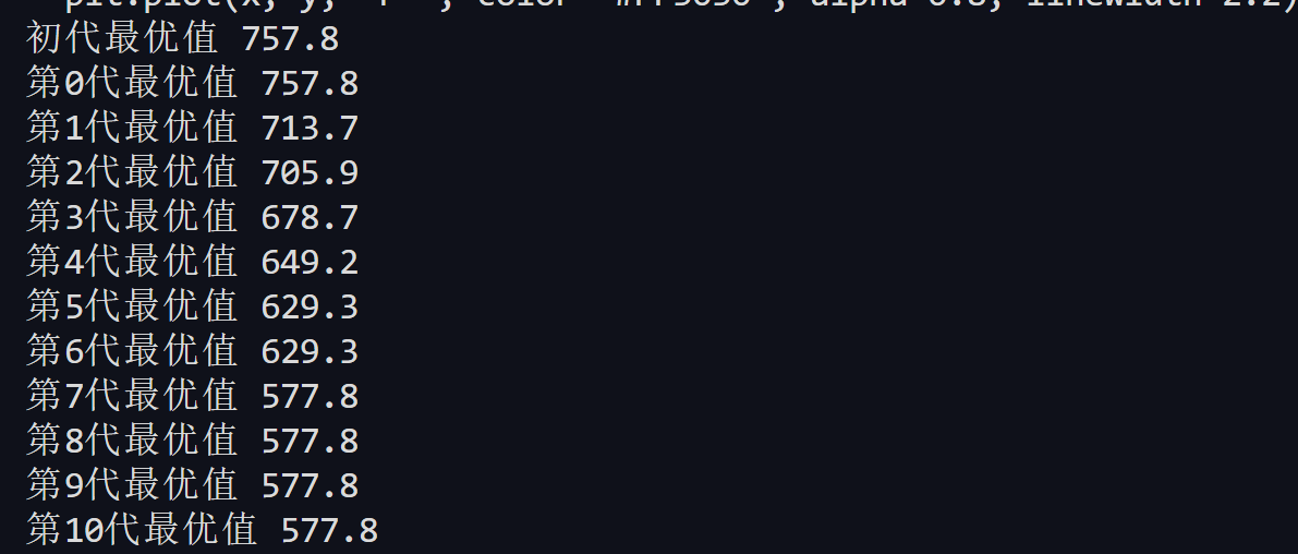
print('初代最优值 %.1f' % (best_fit))
best_fit_list = []
best_fit_list.append(best_fit)

while iteration <= generation:
# 锦标赛赛选择
pop1, fits1 = tournament_select(pops, popsize, fits, tournament_size)
pop2, fits2 = tournament_select(pops, popsize, fits, tournament_size)
# 交叉
child_pops = crossover(popsize, pop1, pop2, pc)
# 变异
child_pops = mutate(child_pops, pm)
# 计算子代适应度
child_fits = [None] * popsize
for i in range(popsize):
child_fits[i] = calFitness(child_pops[i], dis_matrix)
# 一对一生存者竞争
for i in range(popsize):
if fits[i] > child_fits[i]:
fits[i] = child_fits[i]
pops[i] = child_pops[i]

if best_fit > min(fits):
best_fit = min(fits)
best_pop = pops[fits.index(best_fit)]

best_fit_list.append(best_fit)

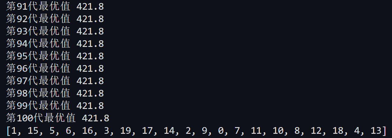
print('第%d代最优值 %.1f' % (iteration, best_fit))
iteration += 1

# 路径顺序
print(best_pop)

draw_path(best_pop, CityCoordinates)

4.2 输出结果

仅展示前10次迭代以及后10次迭代:


DUT人工智能与专家系统_HW2
http://horizongazer.github.io/2024/02/20/DUT人工智能与专家系统_HW2/
作者
HorizonGazer
发布于
2024年2月20日
许可协议