DUT人工智能与专家系统_HW3

1 上机要求

  1. 任选聚类算法和决策树算法中的一种算法编程实现。
  2. 任选BP神经网络和卷积神经网络中的一种模型编程实现手写体识别

2 聚类分析算法

2.1 聚类算法实现(K-Mean)

K-Mean聚类算法是一种简单的迭代型聚类算法,采用距离作为相似性指标,从而发现给定数据集中的K个类,且每个类有一个聚类中心,即质心,每个类的质心是根据类中所有值的均值得到的。

对于给定的一个包含 n个d 维数据点的数据集X及要分得的类别K,选取欧氏距离作为相似度指标。聚类目标是使得各类的聚类平方和最小,即最小化。

Step1 从数据集中随机选择k个数据,作为初始簇的均值向量
Step2 对剩余的每个数据,根据其与各个簇均值向量的距离,将它划分给最近的簇
Step3 在新产生的k个簇的基础上,更新各个簇的均值向量
Step4 重复Step2-Step3,直到停止条件满足,如均值向量不再发生变化,或者达到最大迭代次数等

2.1.1 Python编程实现

1
2
3
4
5
6
7
8
9
10
11
12
13
14
15
16
17
18
19
20
21
22
23
24
25
26
27
28
29
30
31
32
33
34
35
36
37
38
39
40
41
42
import numpy as np  
from sklearn.datasets import make_blobs

import numpy as np

def euclidean_distance(x1, x2):
# 计算两个向量之间的欧氏距离
return np.sum((x1 - x2) ** 2)

def kmeans(X, k, max_iters=100):
# 1. 初始化质心
np.random.seed(0)
indices = np.random.choice(len(X), k, replace=False)
centroids = X[indices]

for _ in range(max_iters):
# 2. 为每个数据点分配最近的质心
labels = np.array([np.argmin([euclidean_distance(x, centroid) for centroid in centroids]) for x in X])

# 3. 更新质心
new_centroids = np.array([X[labels == i].mean(0) for i in range(k)])

# 4. 检查质心是否改变
if np.all(centroids == new_centroids):
break

centroids = new_centroids

return centroids, labels

# 创建一个数据集
X, _ = make_blobs(n_samples=300, centers=4, cluster_std=0.60, random_state=0)

# 运行 K-means 算法
centroids, labels = kmeans(X, k=5)

# 绘制结果
import matplotlib.pyplot as plt

plt.scatter(X[:, 0], X[:, 1], c=labels, cmap='viridis', marker='o', s=50, linewidths=0)
plt.scatter(centroids[:, 0], centroids[:, 1], c='red', marker='x', s=200, linewidths=3)
plt.show()

2.1.2 输出结果

输出结果如下,可知聚类效果较好。

2.2 决策树算法实现(Decision Tree)

决策树(Decision Tree)是一种基本的分类与回归方法。决策树模型呈树形结构,在分类问题中,表示基于特征对数据进行分类的过程。它可以认为是if-then规则的集合。每个内部节点表示在属性上的一个测试,每个分支代表一个测试输出,每个叶节点代表一种类别。

构建决策树的基本步骤

  1. 开始,所有记录看作一个节点
  2. 遍历每个特征的每一种分裂方式,找到最好的分裂特征(分裂点)
  3. 分裂成两个或多个节点
  4. 对分裂后的节点分别继续执行2-3步,直到每个节点足够“纯”为止。如果一个分裂点可以将当前的所有节点分为两类,使得每一类都很“纯”,也就是同一类的记录较多,那么就是一个好分裂点。

下面就以一个经典的打网球的例子来说明如何构建决策树。我们今天是否去打网球(play)主要由天气(outlook)、温度(temperature)、湿度(humidity)、是否有风(windy)来确定。

1
2
3
4
5
6
7
8
9
10
11
12
13
14
15
16
样本中共14条数据。
NO. Outlook temperature humidity windy play
1 sunny hot high FALSE no
2 sunny hot high TRUE no
3 overcast hot high FALSE yes
4 rainy mild high FALSE yes
5 rainy cool normal FALSE yes
6 rainy cool normal TRUE no
7 overcast cool normal TRUE yes
8 sunny mild high FALSE no
9 sunny cool normal FALSE yes
10 rainy mild normal FALSE yes
11 sunny mild normal TRUE yes
12 overcast mild high TRUE yes
13 overcast hot normal FALSE yes
14 rainy mild high TRUE no

2.2.1 Python编程实现

1
2
3
4
5
6
7
8
9
10
11
12
13
14
15
16
17
18
19
20
21
22
23
24
25
26
27
28
29
30
31
32
33
34
35
36
37
38
39
40
41
42
43
44
45
46
47
48
49
50
51
52
53
54
55
56
57
58
59
60
61
62
63
64
65
66
67
68
69
70
71
72
73
74
75
76
77
78
79
80
81
82
83
84
85
86
87
88
89
90
91
92
93
94
95
96
97
98
99
100
101
102
103
104
105
106
107
108
109
110
111
112
113
114
115
116
117
118
119
120
121
122
123
124
125
126
127
128
129
130
131
132
133
134
135
136
137
138
139
140
141
142
143
144
145
146
147
148
149
150
151
152
153
154
155
156
157
158
159
160
161
162
163
164
165
166
167
168
169
170
171
172
173
174
175
176
177
178
179
180
181
182
183
184
185
186
187
188
189
190
191
192
193
194
195
196
197
198
199
200
201
202
203
204
205
206
207
208
209
210
211
212
213
214
215
216
217
218
219
220
221
222
223
224
225
226
227
228
229
230
231
232
233
234
235
236
237
238
239
240
241
242
243
244
245
246
247
248
249
250
251
252
253
254
255
256
257
258
259
260
import math
import operator
import matplotlib as mpl
import matplotlib.pyplot as plt
from pylab import *

mpl.rcParams['font.sans-serif'] = ["SimHei"]
mpl.rcParams['axes.unicode_minus'] = True

def createDataSet():
dataSet=[
['晴','热','高','否','否'],
['晴','热','高','是','否'],
['阴','热','高','否','是'],
['雨','温','高','否','是'],
['雨','凉爽','中','否','是'],
['雨','凉爽','中','是','否'],
['阴','凉爽','中','是','是'],
['晴','温','高','否','否'],
['晴','凉爽','中','否','是'],
['雨','温','中','否','是'],
['晴','温','中','是','是'],
['阴','温','高','是','是'],
['阴','热','中','否','是'],
['雨','温','高','是','否']
]
labels = ['天气','温度','湿度','是否有风'] #两个特征
return dataSet,labels

dataset,dataLabels = createDataSet()

def calcShannonEnt(dataSet):
#样本总个数
totalNum = len(dataSet)
#类别集合
labelSet = {}
#计算每个类别的样本个数
for dataVec in dataSet:
label = dataVec[-1]
if label not in labelSet.keys():
labelSet[label] = 0
labelSet[label] += 1
shannonEnt = 0
#计算熵值
for key in labelSet:
pi = float(labelSet[key])/totalNum
shannonEnt -= pi*math.log(pi,2)
return shannonEnt

#按给定特征划分数据集:返回第featNum个特征其值为value的样本集合,且返回的样本数据中已经去除该特征
def splitDataSet(dataSet, featNum, featvalue):
retDataSet = []
for dataVec in dataSet:
if dataVec[featNum] == featvalue:
splitData = dataVec[:featNum]
splitData.extend(dataVec[featNum+1:])
retDataSet.append(splitData)
return retDataSet
#选择最好的特征划分数据集

def chooseBestFeatToSplit(dataSet):
featNum = len(dataSet[0]) - 1
maxInfoGain = 0
bestFeat = -1
#计算样本熵值,对应公式中:H(X)
baseShanno = calcShannonEnt(dataSet)
#以每一个特征进行分类,找出使信息增益最大的特征
for i in range(featNum):
featList = [dataVec[i] for dataVec in dataSet]
featList = set(featList)
newShanno = 0
#计算以第i个特征进行分类后的熵值,对应公式中:H(X|Y)
for featValue in featList:
subDataSet = splitDataSet(dataSet, i, featValue)
prob = len(subDataSet)/float(len(dataSet))
newShanno += prob*calcShannonEnt(subDataSet)
#ID3算法:计算信息增益,对应公式中:g(X,Y)=H(X)-H(X|Y)
infoGain = baseShanno - newShanno
#C4.5算法:计算信息增益比
#infoGain = (baseShanno - newShanno)/baseShanno
#找出最大的熵值以及其对应的特征
if infoGain > maxInfoGain:
maxInfoGain = infoGain
bestFeat = i
return bestFeat

# 如果决策树递归生成完毕,且叶子节点中样本不是属于同一类,则以少数服从多数原则确定该叶子节点类别
def majorityCnt(labelList):
labelSet = {}
# 统计每个类别的样本个数
for label in labelList:
if label not in labelSet.keys():
labelSet[label] = 0
labelSet[label] += 1
# iteritems:返回列表迭代器
# operator.itemgeter(1):获取对象第一个域的值
# True:降序
sortedLabelSet = sorted(labelSet.items(), key=operator.itemgetter(1), reverse=True)
return sortedLabelSet[0][0]

#创建决策树
def createDecideTree(dataSet, featName):
#数据集的分类类别
classList = [dataVec[-1] for dataVec in dataSet]
#所有样本属于同一类时,停止划分,返回该类别
if len(classList) == classList.count(classList[0]):
return classList[0]
#所有特征已经遍历完,停止划分,返回样本数最多的类别
if len(dataSet[0]) == 1:
return majorityCnt(classList)
#选择最好的特征进行划分
bestFeat = chooseBestFeatToSplit(dataSet)
beatFestName = featName[bestFeat]
del featName[bestFeat]
#以字典形式表示树
DTree = {beatFestName:{}}
#根据选择的特征,遍历该特征的所有属性值,在每个划分子集上递归调用createDecideTree
featValue = [dataVec[bestFeat] for dataVec in dataSet]
featValue = set(featValue)
for value in featValue:
subFeatName = featName[:]
DTree[beatFestName][value] = createDecideTree(splitDataSet(dataSet,bestFeat,value), subFeatName)
return DTree
#print(createDecideTree(dataset,dataLabels))

def getNumLeafs(tree):
numLeafs = 0
#获取第一个节点的分类特征
firstFeat = list(tree.keys())[0]
#得到firstFeat特征下的决策树(以字典方式表示)
secondDict = tree[firstFeat]
#遍历firstFeat下的每个节点
for key in secondDict.keys():
#如果节点类型为字典,说明该节点下仍然是一棵树,此时递归调用getNumLeafs
if type(secondDict[key]).__name__== 'dict':
numLeafs += getNumLeafs(secondDict[key])
#否则该节点为叶节点
else:
numLeafs += 1
return numLeafs

#获取决策树深度
def getTreeDepth(tree):
maxDepth = 0
#获取第一个节点分类特征
firstFeat = list(tree.keys())[0]
#得到firstFeat特征下的决策树(以字典方式表示)
secondDict = tree[firstFeat]
#遍历firstFeat下的每个节点,返回子树中的最大深度
for key in secondDict.keys():
#如果节点类型为字典,说明该节点下仍然是一棵树,此时递归调用getTreeDepth,获取该子树深度
if type(secondDict[key]).__name__ == 'dict':
thisDepth = 1 + getTreeDepth(secondDict[key])
else:
thisDepth = 1
if thisDepth > maxDepth:
maxDepth = thisDepth
return maxDepth
#画出决策树

def createPlot(tree):
# 定义一块画布,背景为白色
fig = plt.figure(1, facecolor='white')
# 清空画布
fig.clf()
# 不显示x、y轴刻度
xyticks = dict(xticks=[], yticks=[])
# frameon:是否绘制坐标轴矩形
createPlot.pTree = plt.subplot(111, frameon=False, **xyticks)
# 计算决策树叶子节点个数
plotTree.totalW = float(getNumLeafs(tree))
# 计算决策树深度
plotTree.totalD = float(getTreeDepth(tree))
# 最近绘制的叶子节点的x坐标
plotTree.xOff = -0.5 / plotTree.totalW
# 当前绘制的深度:y坐标
plotTree.yOff = 1.0
# (0.5,1.0)为根节点坐标
plotTree(tree, (0.5, 1.0), '')
plt.show()

# 定义决策节点以及叶子节点属性:boxstyle表示文本框类型,sawtooth:锯齿形;fc表示边框线粗细
decisionNode = dict(boxstyle="sawtooth", fc="0.5")
leafNode = dict(boxstyle="round4", fc="0.5")

# 定义箭头属性
arrow_args = dict(arrowstyle="<-")


# nodeText:要显示的文本;centerPt:文本中心点,即箭头所在的点;parentPt:指向文本的点;nodeType:节点属性
# ha='center',va='center':水平、垂直方向中心对齐;bbox:方框属性
# arrowprops:箭头属性
# xycoords,textcoords选择坐标系;axes fraction-->0,0是轴域左下角,1,1是右上角
def plotNode(nodeText, centerPt, parentPt, nodeType):
createPlot.pTree.annotate(nodeText, xy=parentPt, xycoords="axes fraction",
xytext=centerPt, textcoords='axes fraction',
va='center', ha='center', bbox=nodeType, arrowprops=arrow_args)

def plotMidText(centerPt, parentPt, midText):
xMid = (parentPt[0] - centerPt[0]) / 2.0 + centerPt[0]
yMid = (parentPt[1] - centerPt[1]) / 2.0 + centerPt[1]
createPlot.pTree.text(xMid, yMid, midText)

def plotTree(tree, parentPt, nodeTxt):
#计算叶子节点个数
numLeafs = getNumLeafs(tree)
#获取第一个节点特征
firstFeat = list(tree.keys())[0]
#计算当前节点的x坐标
centerPt = (plotTree.xOff + (1.0 + float(numLeafs))/2.0/plotTree.totalW, plotTree.yOff)
#绘制当前节点
plotMidText(centerPt,parentPt,nodeTxt)
plotNode(firstFeat,centerPt,parentPt,decisionNode)
secondDict = tree[firstFeat]
#计算绘制深度
plotTree.yOff -= 1.0/plotTree.totalD
for key in secondDict.keys():
#如果当前节点的子节点不是叶子节点,则递归
if type(secondDict[key]).__name__ == 'dict':
plotTree(secondDict[key],centerPt,str(key))
#如果当前节点的子节点是叶子节点,则绘制该叶节点
else:
#plotTree.xOff在绘制叶节点坐标的时候才会发生改变
plotTree.xOff += 1.0/plotTree.totalW
plotNode(secondDict[key], (plotTree.xOff,plotTree.yOff),centerPt,leafNode)
plotMidText((plotTree.xOff,plotTree.yOff),centerPt,str(key))
plotTree.yOff += 1.0/plotTree.totalD

#决策树节点文本可以以中文显示

#创建决策树
myTree = createDecideTree(dataset,dataLabels)
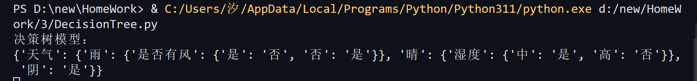
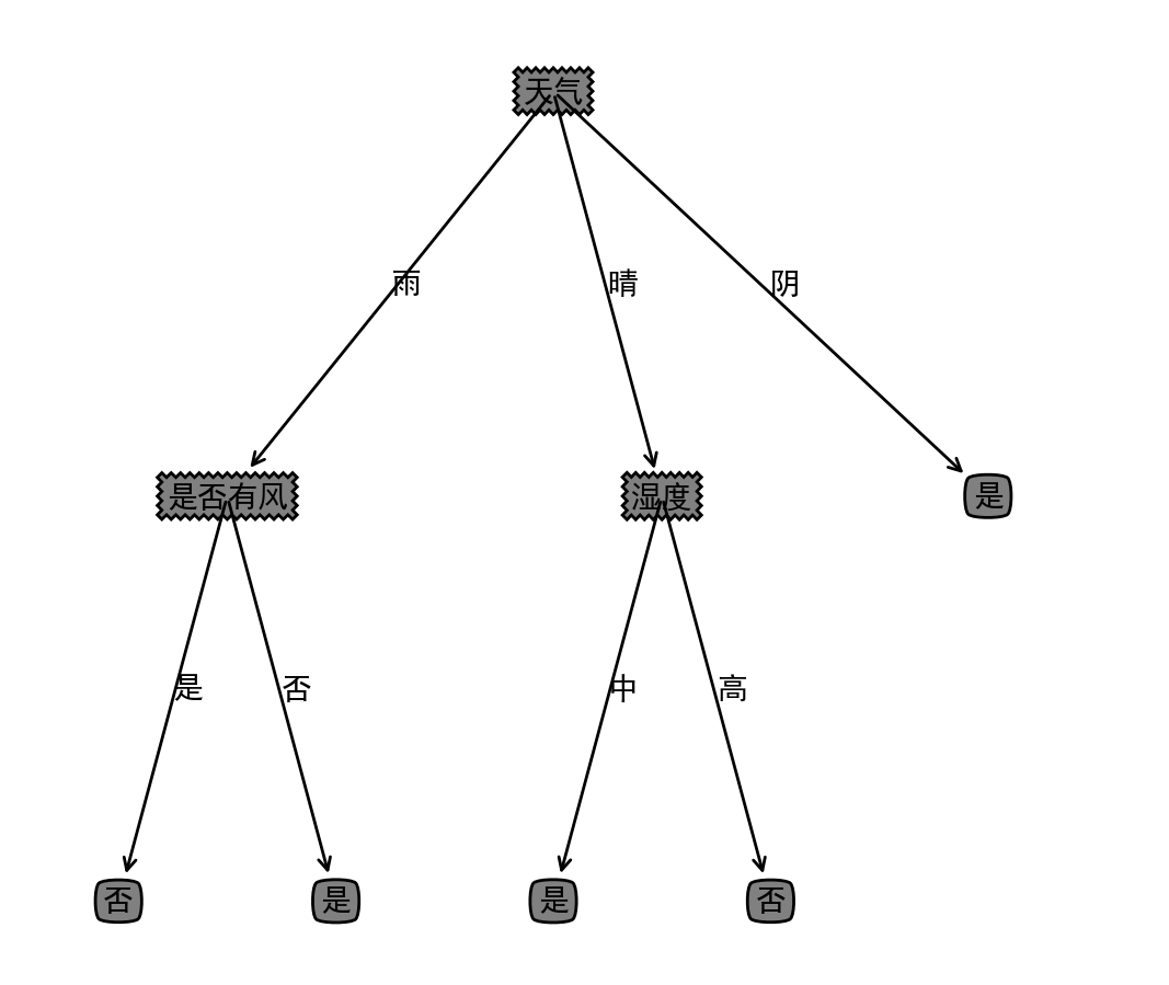
print("决策树模型:")
print(myTree)
createPlot(myTree)

#预测部分
def classify(tree,feat,featValue):
firstFeat = list(tree.keys())[0]
secondDict = tree[firstFeat]
featIndex = feat.index(firstFeat)
for key in secondDict.keys():
if featValue[featIndex] == key:
if type(secondDict[key]).__name__ == 'dict':
classLabel = classify(secondDict[key],feat,featValue)
else:
classLabel = secondDict[key]
return classLabel

feat = ['天气','温度','湿度','是否有风']
dataSet2=[
['晴','温','中','是'],
['阴','温','高','是'],
['阴','热','中','否'],
['雨','温','高','是'],
]

print("预测结果:")
for dataVec2 in dataSet2:
print(classify(myTree,feat,dataVec2))

2.2.2 输出结果

输出结果如下。

3 深度学习

3.1 基于Keras的简单CNN架构的手写体识别

Keras提供了可以很简单地创建卷积神经网络地API。在Keras中实现卷积神经网络,包括卷积层、池化层和全连接层。

  1. 第一个隐藏层是一个称为Conv2D的卷积层。该层使用5×5的感受野,输出具有32个特征图,输入的数据具有input_shape参数所描述的特征,并采用ReLU作为激活函数。
  2. 定义一个采用最大值MaxPooling2D的池化层,并配置它在纵向和横向两个方向的采样因子(pool_size)为2×2,这表示图片在两个维度均变为原来的一半。
  3. 下一层是使用名为Dropout的正则化层,并配置为随机排除层中20%的神经元, 以减少过度拟合。
  4. 将多维数据转换为一维数据的Flatten层。它的输出便于标准的全连接层的处理。
  5. 具有128个神经元的全连接层,采用ReLU作为激活函数。
  6. 输出层有10个神经元,在MNIST数据集的输出具有10个分类,因此采用softmax函数,输出每张图片在每个分类上的得分。

3.1.1 Python编程实现

1
2
3
4
5
6
7
8
9
10
11
12
13
14
15
16
17
18
import tensorflow as tf
import matplotlib.pyplot as plt

# 导入数据集
mnist = tf.keras.datasets.mnist
(train_images, train_labels), (test_images, test_labels) = mnist.load_data()
print("训练集样本及标签", train_images.shape, train_labels.shape)
print("测试集样本及标签", test_images.shape, test_labels.shape)
train_images, test_images = train_images / 255.0, test_images / 255.0 # 归一化,不然梯度爆炸
# 进行绘画
for i in range(15):
plt.subplot(3, 5, i + 1)
plt.xticks([])
plt.yticks([])
plt.grid(False)
plt.imshow(test_images[i])
plt.xlabel(test_labels[i])
plt.show()

1
2
3
4
5
6
7
8
9
10
11
12
13
14
15
16
17
18
19
20
21
22
23
24
25
26
27
28
29
30
31
32
33
34
35
36
37
38
39
40
41
#训练CNN模型
import tensorflow as tf

# 导入数据集
mnist = tf.keras.datasets.mnist
(train_images, train_labels), (test_images, test_labels) = mnist.load_data()
print("训练集样本及标签", train_images.shape, train_labels.shape)
print("测试集样本及标签", test_images.shape, test_labels.shape)
train_images, test_images = train_images / 255.0, test_images / 255.0 # 归一化,不然梯度爆炸

# 建立各层神经网络
model = tf.keras.models.Sequential() # 建立一个堆叠层的神经网络
# 第一卷积层,32卷积核(即32输出通道),卷积核大小5x5,使用Relu激活函数,零值等大填充,输入张量形状28x28,色彩通道为1(即黑白图片)
model.add(tf.keras.layers.Conv2D(32, (5, 5), activation='relu', padding='same', input_shape=(28, 28, 1)))
# 2x2的最大值池化
model.add(tf.keras.layers.MaxPooling2D((2, 2)))
# 第二卷积层,64个输出通道,输入通道这里就不用指定,可以自动承接前一层的
model.add(tf.keras.layers.Conv2D(64, (5, 5), activation='relu', padding='same'))
model.add(tf.keras.layers.MaxPooling2D((2, 2)))
# 扁平化,将二维的张量变成一维,这里28x28经过两次2x2池化,已是7x7大小,现在变成49
model.add(tf.keras.layers.Flatten())
# 全连接层,64个神经元
model.add(tf.keras.layers.Dense(64, activation='relu'))
# dropout层,损失函数0.5
model.add(tf.keras.layers.Dropout(0.5))
# Readout层,输出独热编码
model.add(tf.keras.layers.Dense(10)) # 最后输出10个数

# 编译模型
model.compile(optimizer='adam', # Adam优化器
loss=tf.keras.losses.SparseCategoricalCrossentropy(from_logits=True), # 损失函数
metrics=['accuracy']) # 监控指标:精度
# 开始训练,训练周期8,即将所有训练样本(6万个),遍历八遍,因为输入通道是32个,所以每遍训练1875次,每次32个
model.fit(train_images, train_labels, epochs=8, validation_data=(test_images, test_labels))

# 训练完毕,使用测试集来评估模型精度
test_loss, test_acc = model.evaluate(test_images, test_labels, verbose=2)
print('\n最终测试集上的精度为:', test_acc)

# 保存模型
model.save("CNN模型.h5")

1
2
3
4
5
6
7
8
9
10
11
12
13
14
15
16
17
#使用训练好的卷积神经网络(CNN)模型对前50个测试集图像进行预测的过程。
import tensorflow as tf

# 导入数据集
mnist = tf.keras.datasets.mnist
(train_images, train_labels), (test_images, test_labels) = mnist.load_data()
# 加入待预测的图像及其标签
show_images, show_labels = test_images[0:50], test_labels[0:50]
print("所选取的测试集图片的标签is:", show_labels)
# 引入模型
model = tf.keras.models.load_model("CNN模型.h5")
# 开始预测
predictions = model.predict(show_images)
# 预测完成
predictions_num = tf.argmax(predictions, 1)
# 输出预测标签
print("所预测的标签为:", predictions_num)

1
2
3
4
5
6
7
8
9
10
11
12
13
14
#识别自己的手写体
import tensorflow as tf

# 读取一张自己手写的图片,此处为黑底白字
img_01 = tf.io.read_file('C:/Users/汐/Desktop/手写体.png')
img02 = tf.io.decode_png(img_01, channels=1)
img03 = tf.image.resize(img02, [28, 28])
img = (img03.numpy()).reshape([1, 28, 28])
print("图片转化之后的形状为:", img.shape)
# 运用模型进行预测
model = tf.keras.models.load_model("CNN模型.h5")
predictions = model.predict(img)
predictions_num = tf.argmax(predictions, 1)
print("你的模型认为该数字为:", predictions_num.numpy())

3.1.2 模型测试

输入的手写体为:

模型识别结果为:

3.2 基于Keras的BP手写体识别

反向传播(英语:Backpropagation,缩写为BP)是“误差反向传播”的简称,是一种与最优化方法(如梯度下降法)结合使用的,用来训练人工神经网络的常见方法。该方法对网络中所有权重计算损失函数的梯度。这个梯度会反馈给最优化方法,用来更新权值以最小化损失函数。反向传播要求有对每个输入值想得到的已知输出,来计算损失函数梯度。因此,它通常被认为是一种监督式学习方法。反向传播要求人工神经元(或“节点”)的激励函数可微。

下面举一个简单的例子来介绍什么是梯度下降法以及如何训练神经网络。

假设有这样一个函数(ε是噪声)

BP-func

但我们不知道参数的值,也就是w和b的值,但是我们直到很多(x,y)。那么我们可以通过这些值来预测原函数。

构造如下的损失函数

BP-lossfunc

其中的x和y都是真实值,而w和b是我们要预测的值。我们预测的w和b应该使得损失函数越小越好,这点不难看出,损失函数越小证明我们预测出来的函数越接近真实情况。

BP-chart

假设我们得到的loss函数图像如上图所示,那么我们得目的就是找到一组w和b使得loss函数值处于一个极小值。

BP-dfunc

约定w和b按照上面得式子更新自己的值。其中w和b是原来的值,w’和b’是新值,lr是learning rate的缩写,直观理解就是横坐标移动的程度。根据高等数学的相关知识,我们知道函数梯度的方向指向极大值,所以上面式子用减号,也就达到了梯度下降的目的。梯度下降可以使得loss函数处于极小值。当然处于极小值不一定是处于最小值,可能会造成局部最优解,但这些问题超出了本篇实验报告的讨论范围,所以不作考虑。

经过若干次的更新w和b,我们就会找到一个较小的loss值,也就是说我们找到的w和b就很接近真实值了。

梯度下降是一种常用的优化loss函数的方法,还有其他的方法也可以对loss函数进行优化,例如随机梯度下降、Adagrad、Adam等。

下面介绍应用BP算法完成手写体识别问题。MNIST数据集的每一张图片是一个28x28的矩阵,每个元素是其位置的灰度信息。

我们首先将二维的矩阵打平成一维的,也就是说变成一个784x1的矩阵。上面介绍的简单的例子是单个数字,这里成了矩阵,所以我们的参数也应该是矩阵。

假设我们先将784x1的矩阵乘以一个512x784的矩阵参数,将得到一个512x1的矩阵

再将512x1的矩阵乘以一个256x512的矩阵参数,将得到一个256x1的矩阵

再将256x1的矩阵乘以一个10x256的矩阵参数,将得到一个10x1的矩阵

经过上述操作,我们将一个784x1的矩阵转换成了一个10x1的矩阵。为什么最后要转换成10个元素的矩阵?因为我们的手写体识别问题中有10个数字,最后我们得到的矩阵的每个元素代表的是可能是相应数字的概率。根据得到的概率和实际情况来构造损失函数,再利用梯度下降的方法来更新参数。

上述的好几步的矩阵转换操作实际上就是神经网络中的层,最后一步的10个元素属于输出层,第一次的784x1是输入层,中间的则是隐藏层。

3.2.1 Python编程实现

1
2
3
4
5
6
7
8
9
10
11
12
13
14
15
16
17
18
19
20
21
22
23
24
25
26
27
28
29
30
31
32
33
34
35
36
37
38
39
40
41
42
43
44
45
46
47
48
49
50
51
52
53
54
55
56
57
58
59
60
61
62
63
64
65
66
67
68
import tensorflow as tf
import keras #keras框架导入
from keras.datasets import mnist #数据集
from keras.layers import Dense,Dropout #神经网络层导入
from keras.models import Sequential #模型类型:Sequential序列模型和Model函数模型

#加载mnist数据集,(x_train,y_train)为训练样本, (x_test,y_test)测试样本
(x_train,y_train),(x_test,y_test)=mnist.load_data()
#数据归一化处理,将0~255归一化至 0~1之间,使得数据乘法运算也在0~1之间
x_train=x_train/255.0 #注意是255.0,发生浮点数运算,不是255
x_test=x_test/255.0
#mnist图像数据是28*28矩阵,全连接层是一排一排的数据形状,需要reshape为784(=28*28),
#无论数据结构/shape如何变化,图本身的特征并没有减少。
x_train=x_train.reshape(60000,784).astype('float32') #训练数据集60000个
x_test=x_test.reshape(10000,784).astype('float32') #测试数据集10000个

#标签转one hot操作,将所有数据从1,2,3,4,...标注改编为
# 如 1 表达为【0,1,0,0,0,0,0,0,0,0】
# 如 5 表达为【0,0,0,0,0,1,0,0,0,0】
y_train=keras.utils.to_categorical(y_train,num_classes=10) #10个类别
y_test =keras.utils.to_categorical(y_test,num_classes=10)

#搭建网络模型---全连接层
model=Sequential() #模型实例化
#向模型中添加Dense层为全连接层--类似面向过程的编程
#第一隐含层,untils为神经元个数(不能太大),input_shape为输入层输入结构,activation激活函数
model.add(Dense(units=128,input_shape=(784,),activation='relu'))
#第二层,这里不需要input_shape,自动以第一层结果作为输入
model.add(Dense(units=128,activation='relu'))
#为防止过拟合,添加Dropout层,表示从所有学习的特征中随机扔掉25%不要,以预防前面过度学习。
model.add(Dropout(0.25))
#输出层,手写数字共0~9十个类别
model.add(Dense(units=10,activation='softmax'))

#模型编译---训练设置
model.compile(loss='categorical_crossentropy',optimizer='adam',metrics=['accuracy'])
#启动训练
model.fit(
x=x_train,
y=y_train,
batch_size=64,#每轮都是60000个样本,但不能将6万样本一次训练,那样所需内存过大,所以设置batch_size为每次训练样本数
epochs=10,#训练多少轮次
)
#模型测试
loss,acc=model.evaluate(x_test,y_test)
print(loss,acc)
#模型保存 --*.h5格式
model.save('mnistTrain.h5')

#下面是测试代码
#应用模型测试
from PIL import Image
from keras.models import load_model
import numpy as np
import matplotlib.pyplot as plt
#加载要测试的数字图像
img_photo=Image.open('屏幕截图 2024-05-04 200823.png')
#统一数字图像大小为28*28
img_gray=img_photo.convert('L')
img_to_array=np.array(img_gray.resize((28,28)))
#将数字图像矩阵数改为一排并归一化
img_to_array=img_to_array.reshape(1,784)/255.0
#加载模型
model=load_model('mnistTrain.h5')
#进行预测
prediction=model.predict(img_to_array)
#输出预测值中最大概率对应下标即为所预测数字
print(np.argmax(prediction))

3.2.2 模型测试

输入手写体:

输出:

可见该模型识别手写体的准确性并不高。


DUT人工智能与专家系统_HW3
http://horizongazer.github.io/2024/03/05/DUT人工智能与专家系统_HW3/
作者
HorizonGazer
发布于
2024年3月5日
许可协议