一篇基于R语言的scRNA-seq文章复现

1 文章概述

文章标题:Comprehensive single-cell transcriptomic and proteomic analysis reveals NK cell exhaustion and unique tumor cell evolutionary trajectory in non-keratinizing nasopharyngeal carcinoma

2023年发表于Journal of Translational Medicine,IF=7.4

2 文章实验设计

目的:研究NK细胞和肿瘤细胞在非角化性鼻咽癌(NK-NPC)中的作用,NK-NPC与EBV感染密切相关

方法:收集3例NK-NPC样本和3例正常鼻咽黏膜样本进行蛋白质组分析,联合GSE162025(NK-NPC单细胞转录组数据)和GSE150825(NLH单细胞转录组数据)进行分析

分析步骤:

  1. 对蛋白组数据进行分析,发现NK细胞介导的细胞毒性相关蛋白显著下调,NK细胞功能可能受到抑制。

  2. 免疫组化发现NK-NPC样本中,与NK细胞相关的B2M,CD56+,Granzyme B均下调

  3. 对NK-NPC单细胞转录组样本进行分析,T细胞,B细胞,NK细胞在所有类型的细胞中排名前三

  4. 对NK细胞取子集进行细分,得到1个mast cell和3个NK细胞cluster,从NK细胞毒性激活/抑制,细胞通讯,NK细胞功能相关的标志物,NK细胞介导的毒性通路等角度进行分析,并用NLH单细胞转录数据集进行验证

  5. 对上皮细胞取子集进行细分,用copykat鉴定良性和恶性上皮细胞,对恶性上皮细胞再进行细分,得到tumor1和tumor2两类,考察多个关键基因,发现EBV感染可能与tumor1相关

  6. 对tumor1再取子集,得到4个cluster,用拟时序分析4个cluster之间的演变过程,分析了关键基因和通路在不同cluster之间的变化,推测EBV感染的机制

3 复现前准备

3.1 数据

数据 数据说明 来源
12967_2023_4112_MOESM1_ESM.xlsx NK-NPC蛋白质组学结果 文献附件
GSE162025_RAW 使用单细胞转录组和 T 细胞受体测序对分析来自 10 对 NPC 肿瘤血对的 176,447 个细胞 https://www.ncbi.nlm.nih.gov/geo/query/acc.cgi?acc=GSE162025
GSE150825_RAW(barcodes.tsv.gz, features.tsv.gz, matrix.mtx.gz) 鼻咽癌微环境的单细胞转录组分析和免疫谱分析 https://www.ncbi.nlm.nih.gov/geo/query/acc.cgi?&acc=GSE150825

3.2 平台和软件

1
platform       x86_64-w64-mingw32   
软件 版本
R 4.3.1
RStudio 2024.04.0

4 复现流程

4.1 导入包

1
2
3
4
5
6
7
8
9
10
11
12
13
14
15
16
17
18
19
20
21
22
23
if(T){
library(Seurat)
library(data.table)
library(stringr)
library(readxl)
library(tibble)
library(limma)
library(dplyr)
library(ggplot2)
library(ggrepel)
library(pheatmap)
library(clusterProfiler)
library(org.Hs.eg.db)
library(tidyverse)
library(scRNAtoolVis)
library(enrichplot)
library(GSEABase)
library(msigdbr)
library(CellChat)
library(copykat)
library(patchwork)
library(SCORPIUS)
}

4.2 NK-NPC蛋白质组学分析

1
2
3
4
5
6
7
8
9
10
11
12
13
14
15
16
17
18
19
20
21
22
23
24
25
26
27
28
29
30
31
32
33
34
35
36
37
38
39
40
41
42
43
44
45
46
47
48
49
50
51
52
53
54
55
56
57
58
59
60
61
62
63
64
setwd("C:\\Users\\汐\\Desktop\\R语言复现\\NK细胞耗竭和肿瘤细胞进化轨迹")

# proteomics
data_pro <- read_xlsx('rawdata/12967_2023_4112_MOESM1_ESM.xlsx')
data_pro <- data_pro[,c(23,37:42)]
colnames(data_pro) <- c('gene symbol','NK_NPC-1','NK_NPC-2','NK_NPC-3','normal-1','normal-2','normal-3')
data_pro$`gene symbol` <- str_split(data_pro$`gene symbol`,';',simplify = T)[,1]
data_pro <- data_pro[!duplicated(data_pro$`gene symbol`),]
data_pro <- data_pro[!is.na(data_pro$`gene symbol`),]
data_pro <- column_to_rownames(data_pro,'gene symbol')
data_pro <- data_pro[rowSums(!is.na(data_pro))==6,]
# deg
input_matrix <- log2(data_pro)
group <- as.factor(rep(c('NK_NPC','normal'),each=3))
design <- model.matrix(~0+group)
colnames(design) <- c('NK_NPC','normal')
rownames(design) <- colnames(input_matrix)
fit <- lmFit(input_matrix,design)
con.matrix <- makeContrasts('NK_NPC-normal',levels = design)
fit2 <- contrasts.fit(fit,contrasts = con.matrix)
fit2 <- eBayes(fit2)
# 差异筛选
options(digits = 4)
deg <- topTable(fit2,n=Inf)
up <- (deg$logFC>0.5)&(deg$P.Val<0.05)
down <- (deg$logFC<(-0.5))&(deg$P.Val<0.05)
change <- ifelse(up,'up',ifelse(down,'down','none'))
deg <- mutate(deg,change)
deg <- mutate(deg,'p' = -log10(deg$P.Val))
top5 <- rownames(top_n(deg[deg$change=='up',],5,logFC))
down5 <- rownames(top_n(deg[deg$change=='down',],-5,logFC))
deg$label <- ifelse(rownames(deg) %in% c(top5,down5),rownames(deg),NA)
# volcano
ggplot(deg,aes(x=logFC,y=p,color=change))+
geom_point()+
geom_vline(xintercept = 1,linetype=2,color='gray',linewidth=1)+
geom_vline(xintercept = -1,linetype=2,color='gray',linewidth=1)+
geom_hline(yintercept = -log10(0.05),linetype=2,color='gray',linewidth=1)+
geom_text_repel(aes(logFC,label=label),
max.overlaps = 100000,size=3,segment.color='black',
box.padding=unit(1,'lines'))
# 差异蛋白pca
pca_data <- data_pro[rownames(deg[deg$change!='none',]),]
pca <- prcomp(t(log2(pca_data)),scale. = T)
xlab <- paste0('PCA_1(', round(summary(pca)$importance[2,1]*100,2),'%)')
ylab <- paste0('PCA_2(', round(summary(pca)$importance[2,2]*100,2),'%)')
ggplot(data.frame(pca$x),aes(x=PC1,y=PC2,color=group))+
geom_point(size = 3)+stat_ellipse(level = 0.95, show.legend = F)+
labs(x = xlab,y = ylab,title = 'PCA Analysis')+
theme(plot.title = element_text(hjust = 0.5))+
guides(color = guide_legend(title = 'Group'))
# heatmap
NK_cytotoxicity <- c('PRKCB','PTPN11','LCK','ITGAL','PIK3CB','MAPK3','CASP3')
pheatmap(data_pro[NK_cytotoxicity,],scale = 'row')
# KEGG
kegg_id <- bitr(rownames(deg[deg$change!='none',]),fromType = 'SYMBOL',toType = 'ENTREZID',OrgDb = org.Hs.eg.db)
kegg <- enrichKEGG(kegg_id$ENTREZID,'hsa',keyType = 'kegg')
kegg <- setReadable(kegg,OrgDb = org.Hs.eg.db,keyType = 'ENTREZID')
fc <- deg[deg$change!='none','logFC']
names(fc) <- rownames(deg[deg$change!='none',])
cnetplot(kegg,color.params = list(foldChange = fc,edge=T))

rm(list = ls())
gc()
Fig1.A_Volcano

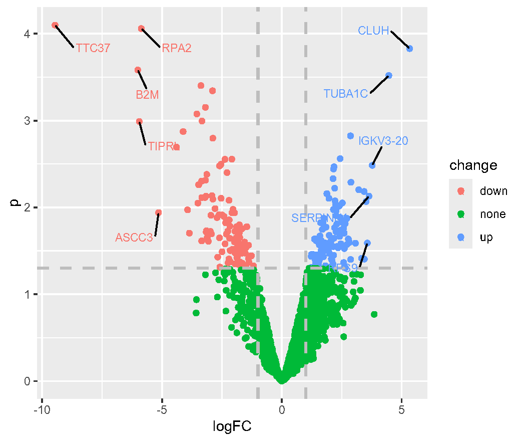
Fig.1.A NK-NPC蛋白质组学差异分析结果的火山图,与正常组相比,NK-NPC组有76种蛋白上调,85种蛋白下调,并标记了几个有趣的蛋白

Fig1.B_PCA

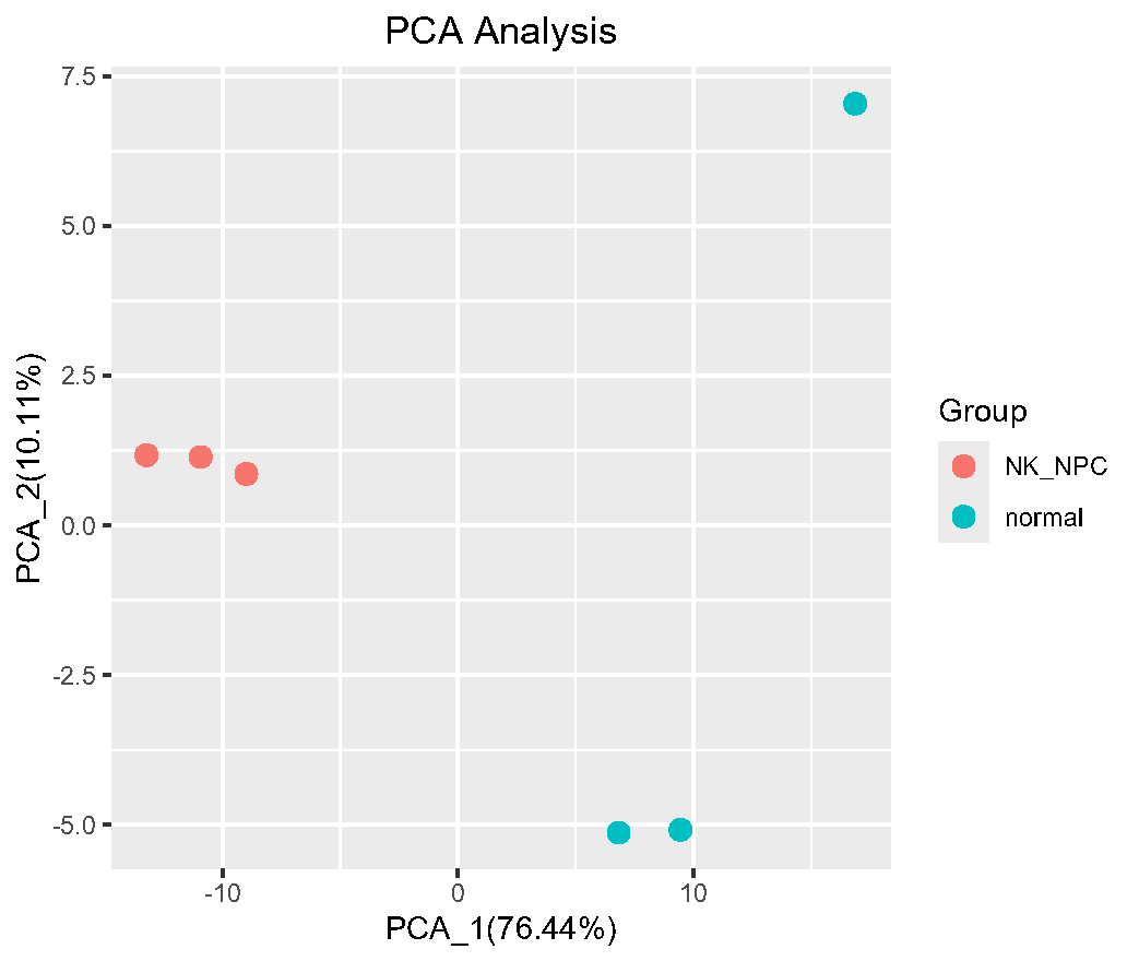
Fig.1.B 主成分分析(PCA)可很好地区分3个NK-NPC和3个正常鼻咽组织之间的差异表达蛋白。

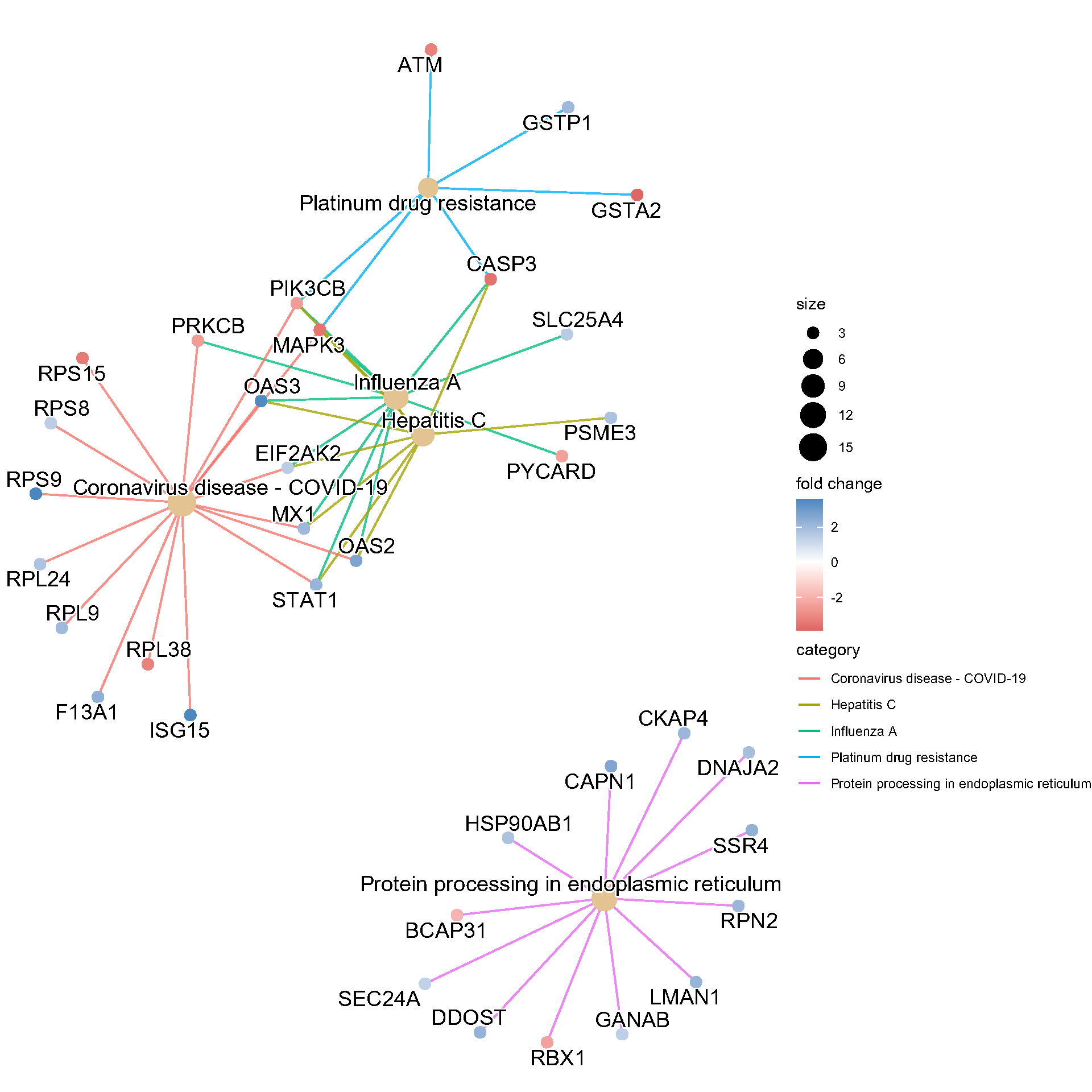
Fig.1.C 对 161 种差异表达蛋白进行 KEGG 富集分析。

Fig1.D_Heatmap

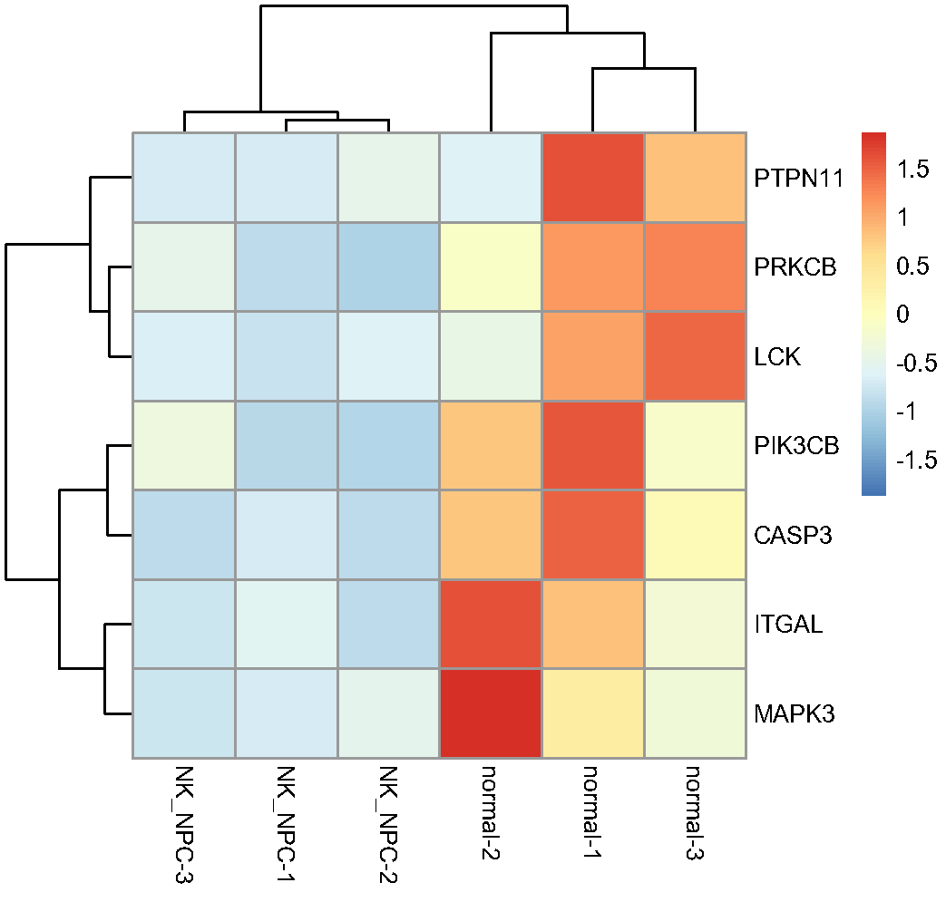
Fig.1.D 蛋白热图显示,富集在自然杀伤细胞介导的细胞毒性通路中的DE蛋白在NK-NPC组中显著下调,包括PRKCB、PTPN11、LCK、ITGAL、PIK3CB、CASP3和MAPK3。

4.3 GSE162025的scRNA-seq分析

1
2
3
4
5
6
7
8
9
10
11
12
13
14
15
16
17
18
19
20
21
22
23
24
25
26
27
28
29
30
31
32
33
34
35
36
37
38
39
40
41
42
43
44
45
46
47
48
49
50
51
52
53
54
55
56
57
58
59
60
61
62
63
64
65
66
67
68
69
70
71
72
73
74
75
# 数据读取
setwd("C:\\Users\\汐\\Desktop\\R语言复现\\NK细胞耗竭和肿瘤细胞进化轨迹")
# 162025
data_162025 <- fread('rawdata/GSE162025_RAW/Tumor/GSM4929846_NPC_SC_1802_Tumor_count.csv.gz')

filename <- paste('rawdata/GSE162025_RAW/Tumor/',list.files('rawdata/GSE162025_RAW/Tumor/'),sep = '')
data_162025List <- lapply(filename, function(x){
obj <- CreateSeuratObject(counts = read.csv(x),
# project = paste(str_split(str_split(x,'/')[[1]][3],'_')[[1]][2:4],collapse = '_'),
min.cells = 3, min.features = 200)
})

data_162025 <- merge(data_162025List[[1]],data_162025List[-1],add.cell.ids = names(data_162025List))
data_162025$orig.ident <- apply(str_split(rownames(data_162025@meta.data),'_',simplify = T)[,1:3],
1,
function(x){paste0(x,collapse ='_')})

dim(data_162025)
saveRDS(data_162025,file = 'data_162025.RDS')
data_162025 <- readRDS('data_162025.RDS')

# QC
#VlnPlot(data_162025,features = 'nFeature_RNA',group.by = 'orig.ident',pt.size = 0)
data_162025 <- subset(data_162025,subset = nFeature_RNA>200 & nFeature_RNA<4000)

data_162025 <- PercentageFeatureSet(data_162025,pattern = '^MT',col.name = 'percent.MT')
#VlnPlot(data_162025,features = 'percent.MT',group.by = 'orig.ident',pt.size = 0)
data_162025 <- subset(data_162025,subset = percent.MT<5)
dim(data_162025)
# 降维
data_162025 <- NormalizeData(data_162025)
data_162025 <- FindVariableFeatures(data_162025)
data_162025 <- ScaleData(data_162025)
data_162025 <- RunPCA(data_162025)
#ElbowPlot(data_162025,ndims = 30)
# 分群
data_162025 <- RunTSNE(data_162025,reduction = 'pca',dims = 1:20)
#DimPlot(data_162025,reduction = 'tsne',label = T,group.by = 'orig.ident')
data_162025 <- FindNeighbors(data_162025,dims = 1:20)
data_162025 <- FindClusters(data_162025,resolution = 0.8)
#DimPlot(data_162025,reduction = 'tsne',label = T,group.by = 'seurat_clusters')

# 注释
# T cell ['PTPRC','CD3D','CD8A']---[0,1,3,4,5,7,8,9,10,11,12,13]
# NK cell ['PTPRC','NKG7','CD96','KLRC1','NCAM1']---[7,11] [0,1,5,7,10,11,13]
# Myeloid cells ['CD14', 'CD68', 'CD163', 'ITGAX','FCGR3A']---[15,18,19]
# Epithelial cells ['EPCAM', 'KRT5', 'TP63', 'SSTR2']---[16]
# B cell ['CD19', 'MS4A1', 'CD79A']---[2,6,14,17]
# mast cell ['TPSAB1','TPSB2','CPA3'] --- [20]


data_162025@meta.data[data_162025@meta.data$seurat_clusters %in% c(0,1,3,4,5,7,8,9,10,11,12,13),'type'] <- 'T cells'
data_162025@meta.data[data_162025@meta.data$seurat_clusters %in% c(7,11,20),'type'] <- 'NK cell'
data_162025@meta.data[data_162025@meta.data$seurat_clusters %in% c(15,18,19),'type'] <- 'Myeloid cells'
data_162025@meta.data[data_162025@meta.data$seurat_clusters %in% c(16),'type'] <- 'Epithelial cells'
data_162025@meta.data[data_162025@meta.data$seurat_clusters %in% c(2,6,14,17),'type'] <- 'B cells'
saveRDS(data_162025,file = 'data_162025_type.RDS')
data_162025 <- readRDS('data_162025_type.RDS')
DimPlot(data_162025,reduction = 'tsne',label = T,group.by = 'type')
# 细胞类型占比堆叠柱状图
cell_ratio <- matrix(nrow = length(unique(data_162025@meta.data$type)),
ncol = length(unique(data_162025@meta.data$orig.ident)))
cell_ratio <- as.data.frame(cell_ratio,row.names = unique(data_162025@meta.data$type))
colnames(cell_ratio) <- unique(data_162025@meta.data$orig.ident)
table(data_162025@meta.data$orig.ident)
for (cell in unique(data_162025@meta.data$type)){
cell_count <- sum(data_162025@meta.data$type==cell)
for (sample in unique(data_162025@meta.data$orig.ident)){
cell_ratio[cell,sample] <- sum(data_162025@meta.data$type==cell & data_162025@meta.data$orig.ident==sample) / cell_count
}
}
cell_ratio <- rownames_to_column(cell_ratio,var = 'cell_type')
cell_ratio <- pivot_longer(cell_ratio,cols = -cell_type,names_to = 'sample')
ggplot(cell_ratio, aes( x = cell_type, weight = value, fill = sample))+
geom_bar( position = "stack")+coord_flip()

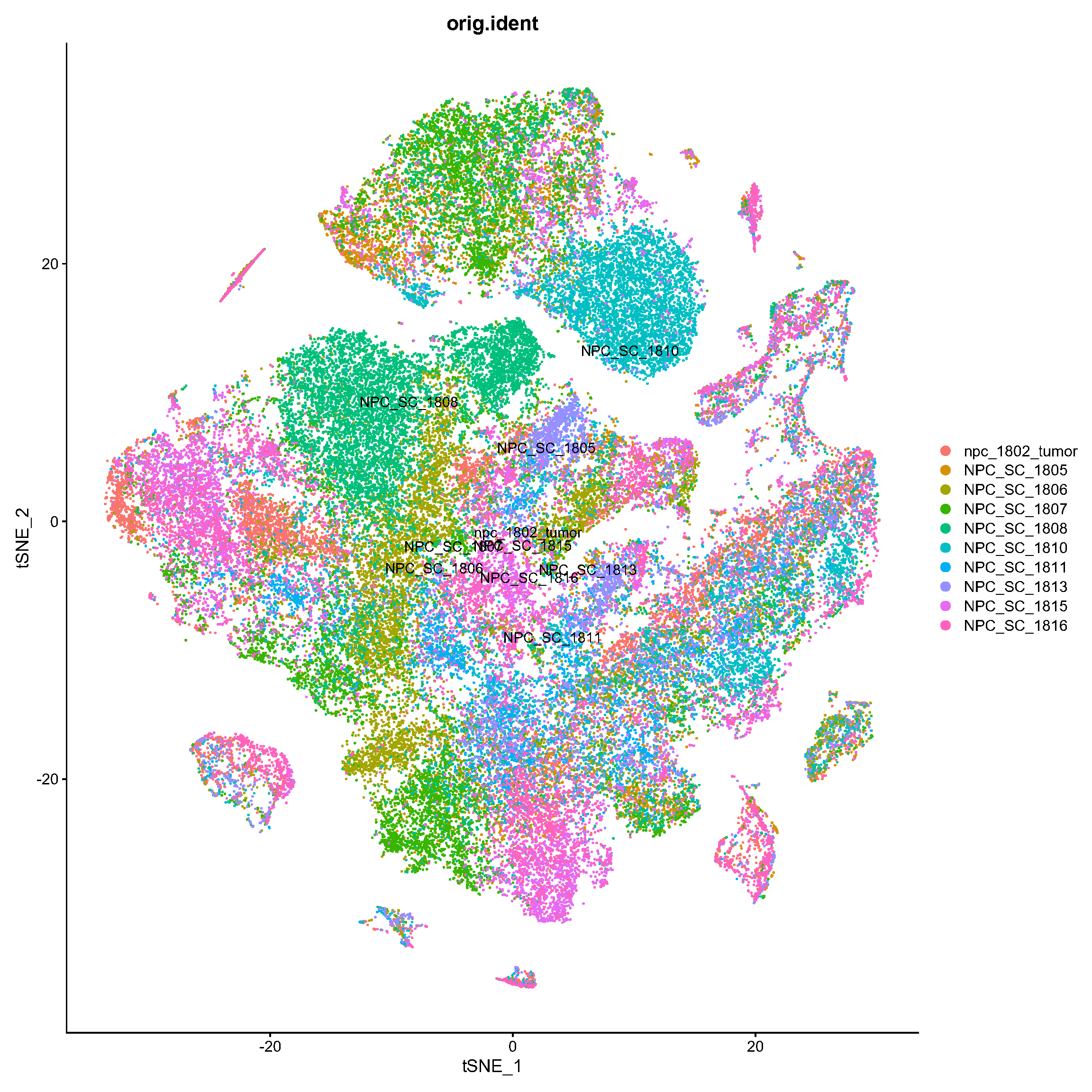
Fig.2.A NK-NPC单细胞图谱。通过降维和聚类 79,000 个细胞获得了 19 个簇。

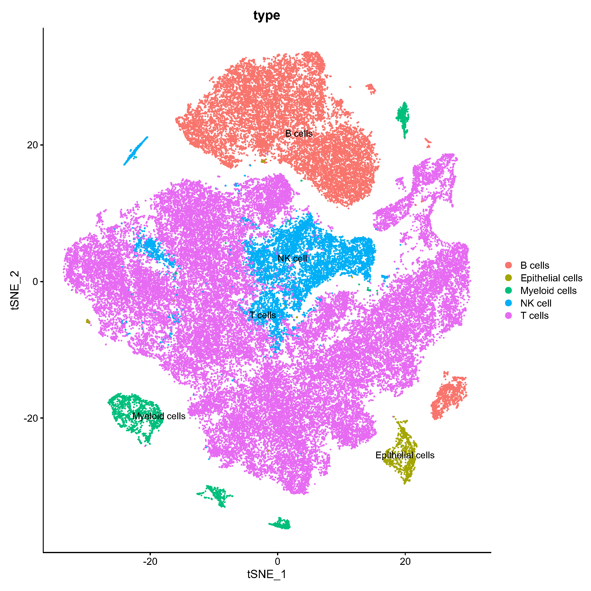
Fig.2.B 19个簇通过其各自的标记基因被识别为不同类型的细胞:上皮细胞、T细胞、NK细胞、髓样细胞和B细胞。

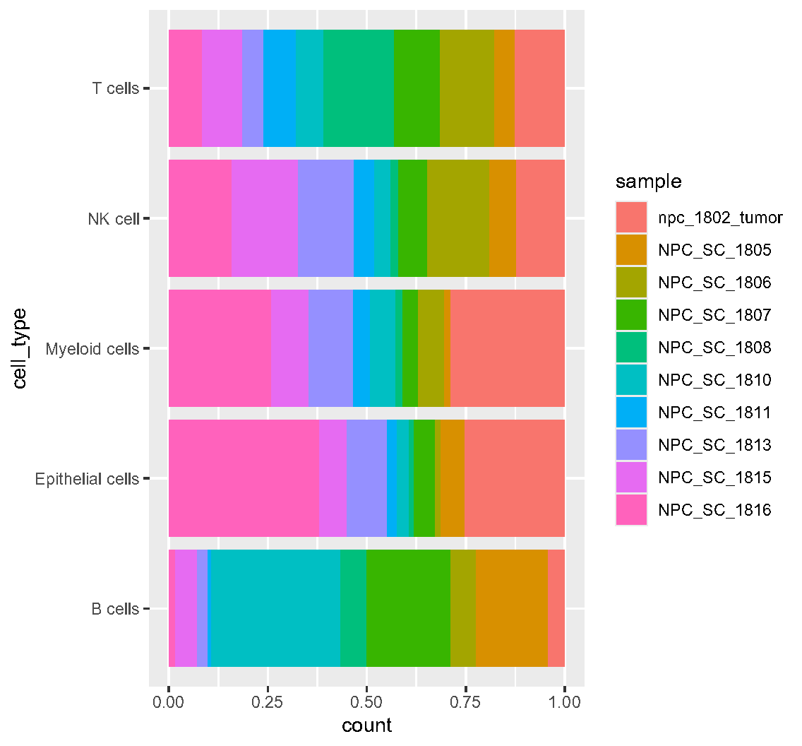
Fig.2.D 10 个样本中每个样本中细胞类型比例的条形图

4.4 NK细胞亚型分析和衰竭情况

1
2
3
4
5
6
7
8
9
10
11
12
13
14
15
16
17
18
19
20
21
22
23
24
25
26
27
28
29
30
31
32
33
34
35
36
37
38
39
40
41
42
43
44
45
46
47
48
49
50
51
52
53
54
55
56
57
58
59
60
61
62
63
64
65
66
67
68
69
70
71
72
73
74
75
76
77
78
79
80
81
82
83
84
85
86
87
88
89
90
91
92
93
94
95
# 对NK细胞继续细分
NK_subtype <- subset(data_162025,subset= type == 'NK cell')
NK_subtype <- NormalizeData(NK_subtype)
NK_subtype <- FindVariableFeatures(NK_subtype)
NK_subtype <- ScaleData(NK_subtype)
NK_subtype <- RunPCA(NK_subtype)
ElbowPlot(NK_subtype,ndims = 30)
NK_subtype <- RunTSNE(NK_subtype,reduction = 'pca',dims = 1:10)
DimPlot(NK_subtype,reduction = 'tsne')
NK_subtype <- FindNeighbors(NK_subtype,dims = 1:10)
NK_subtype <- FindClusters(NK_subtype,resolution = 0.15)
DimPlot(NK_subtype,reduction = 'tsne',group.by = 'seurat_clusters',label = T)
NK_subtype$type <- ifelse(NK_subtype$seurat_clusters=='0','NK1',
ifelse(NK_subtype$seurat_clusters=='1','NK2',
ifelse(NK_subtype$seurat_clusters=='2','NK3',
ifelse(NK_subtype$seurat_clusters=='3','NK4','mast'))))
DimPlot(NK_subtype,reduction = 'tsne',group.by = 'type',label = T)
# scRNA volcano
NK_deg <- FindAllMarkers(NK_subtype)
NK_deg$cluster <- ifelse(NK_deg$cluster=='0','NK1',
ifelse(NK_deg$cluster=='1','NK2',
ifelse(NK_deg$cluster=='2','NK3','NK4')))
jjVolcano(NK_deg)
saveRDS(NK_subtype,file = 'NK_subtype.RDS')
# GSEA
NK_1df <- NK_deg[NK_deg$cluster=='NK1',]

NK_1_up <- NK_1df[NK_1df$avg_log2FC>0.25 & NK_1df$p_val_adj<0.05,'avg_log2FC']
names(NK_1_up) <- bitr(NK_1df[NK_1df$avg_log2FC>0.25 & NK_1df$p_val_adj<0.05,'gene'],
fromType = 'SYMBOL',toType = 'ENTREZID',OrgDb = org.Hs.eg.db)[,'ENTREZID']
NK_1_up <- sort(NK_1_up,decreasing = T)
NK_1_up_gse <- gseKEGG(NK_1_up)
dim(NK_1_up_gse@result)

NK_1_down <- NK_1df[NK_1df$avg_log2FC<(-0.25) & NK_1df$p_val_adj<0.05,'avg_log2FC']
names(NK_1_down) <- bitr(NK_1df[NK_1df$avg_log2FC<(-0.25) & NK_1df$p_val_adj<0.05,'gene'],
fromType = 'SYMBOL',toType = 'ENTREZID',OrgDb = org.Hs.eg.db)[,'ENTREZID']
NK_1_down <- sort(NK_1_down,decreasing = T)
NK_1_down_gse <- gseKEGG(NK_1_down)
dim(NK_1_down_gse@result)

gseaplot2(NK_1_up_gse,geneSetID = 1:6,title = 'NK1')
############ NK2
NK_2df <- NK_deg[NK_deg$cluster=='NK2',]

NK_2_up <- NK_2df[NK_2df$avg_log2FC>0.25 & NK_2df$p_val_adj<0.05,'avg_log2FC']
names(NK_2_up) <- bitr(NK_2df[NK_2df$avg_log2FC>0.25 & NK_2df$p_val_adj<0.05,'gene'],
fromType = 'SYMBOL',toType = 'ENTREZID',OrgDb = org.Hs.eg.db)[,'ENTREZID']
NK_2_up <- sort(NK_2_up,decreasing = T)
NK_2_up_gse <- gseKEGG(NK_2_up)

NK_2_down <- NK_2df[NK_2df$avg_log2FC<(-0.25) & NK_2df$p_val_adj<0.05,'avg_log2FC']
names(NK_2_down) <- bitr(NK_2df[NK_2df$avg_log2FC<(-0.25) & NK_2df$p_val_adj<0.05,'gene'],
fromType = 'SYMBOL',toType = 'ENTREZID',OrgDb = org.Hs.eg.db)[,'ENTREZID']
NK_2_down <- sort(NK_2_down,decreasing = T)
NK_2_down_gse <- gseKEGG(NK_2_down)
dim(NK_2_down_gse@result)

gseaplot2(NK_2_down_gse,geneSetID = 1:8,title = 'NK2')
############ NK3
NK_3df <- NK_deg[NK_deg$cluster=='NK3',]

NK_3_up <- NK_3df[NK_3df$avg_log2FC>0.25 & NK_3df$p_val_adj<0.05,'avg_log2FC']
names(NK_3_up) <- bitr(NK_3df[NK_3df$avg_log2FC>0.25 & NK_3df$p_val_adj<0.05,'gene'],
fromType = 'SYMBOL',toType = 'ENTREZID',OrgDb = org.Hs.eg.db)[,'ENTREZID']
NK_3_up <- sort(NK_3_up,decreasing = T)
NK_3_up_gse <- gseKEGG(NK_3_up)
dim(NK_3_up_gse@result)

NK_3_down <- NK_3df[NK_3df$avg_log2FC<(-0.25) & NK_3df$p_val_adj<0.05,'avg_log2FC']
names(NK_3_down) <- bitr(NK_3df[NK_3df$avg_log2FC<(-0.25) & NK_3df$p_val_adj<0.05,'gene'],
fromType = 'SYMBOL',toType = 'ENTREZID',OrgDb = org.Hs.eg.db)[,'ENTREZID']
NK_3_down <- sort(NK_3_down,decreasing = T)
NK_3_down_gse <- gseKEGG(NK_3_down)
dim(NK_3_down_gse@result)
gseaplot2(NK_3_up_gse,geneSetID = 1,title = NK_3_up_gse@result$Description)
gseaplot2(NK_3_down_gse,geneSetID = 1:8,title = 'NK3')
############ NK4
NK_4df <- NK_deg[NK_deg$cluster=='NK4',]

NK_4_up <- NK_4df[NK_4df$avg_log2FC>0.25 & NK_4df$p_val_adj<0.05,'avg_log2FC']
names(NK_4_up) <- bitr(NK_4df[NK_4df$avg_log2FC>0.25 & NK_4df$p_val_adj<0.05,'gene'],
fromType = 'SYMBOL',toType = 'ENTREZID',OrgDb = org.Hs.eg.db)[,'ENTREZID']
NK_4_up <- sort(NK_4_up,decreasing = T)
NK_4_up_gse <- gseKEGG(NK_4_up)
dim(NK_4_up_gse@result)

NK_4_down <- NK_4df[NK_4df$avg_log2FC<(-0.25) & NK_4df$p_val_adj<0.05,'avg_log2FC']
names(NK_4_down) <- bitr(NK_4df[NK_4df$avg_log2FC<(-0.25) & NK_4df$p_val_adj<0.05,'gene'],
fromType = 'SYMBOL',toType = 'ENTREZID',OrgDb = org.Hs.eg.db)[,'ENTREZID']
NK_4_down <- sort(NK_4_down,decreasing = T)
NK_4_down_gse <- gseKEGG(NK_4_down)
dim(NK_4_down_gse@result)

gseaplot2(NK_4_down_gse,geneSetID = 1:4)

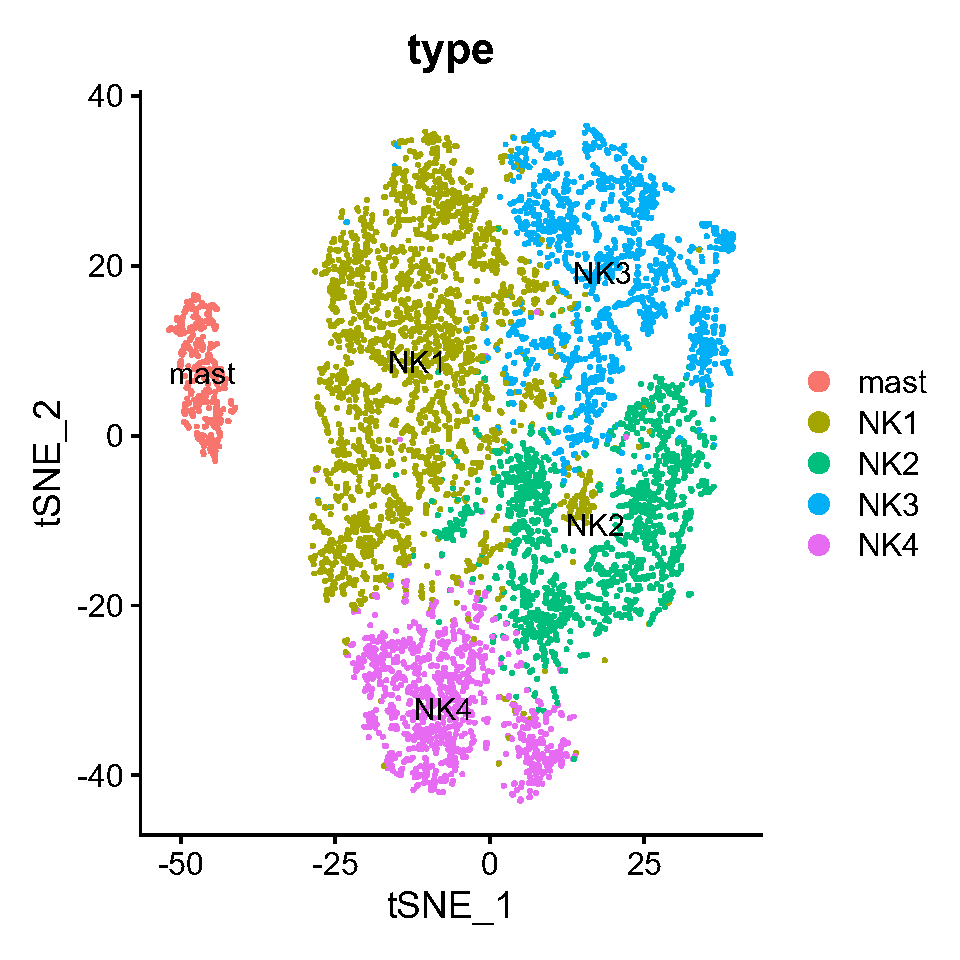
Fig.3.A 通过NK细胞的降维和聚类获得NK1-4细胞亚群

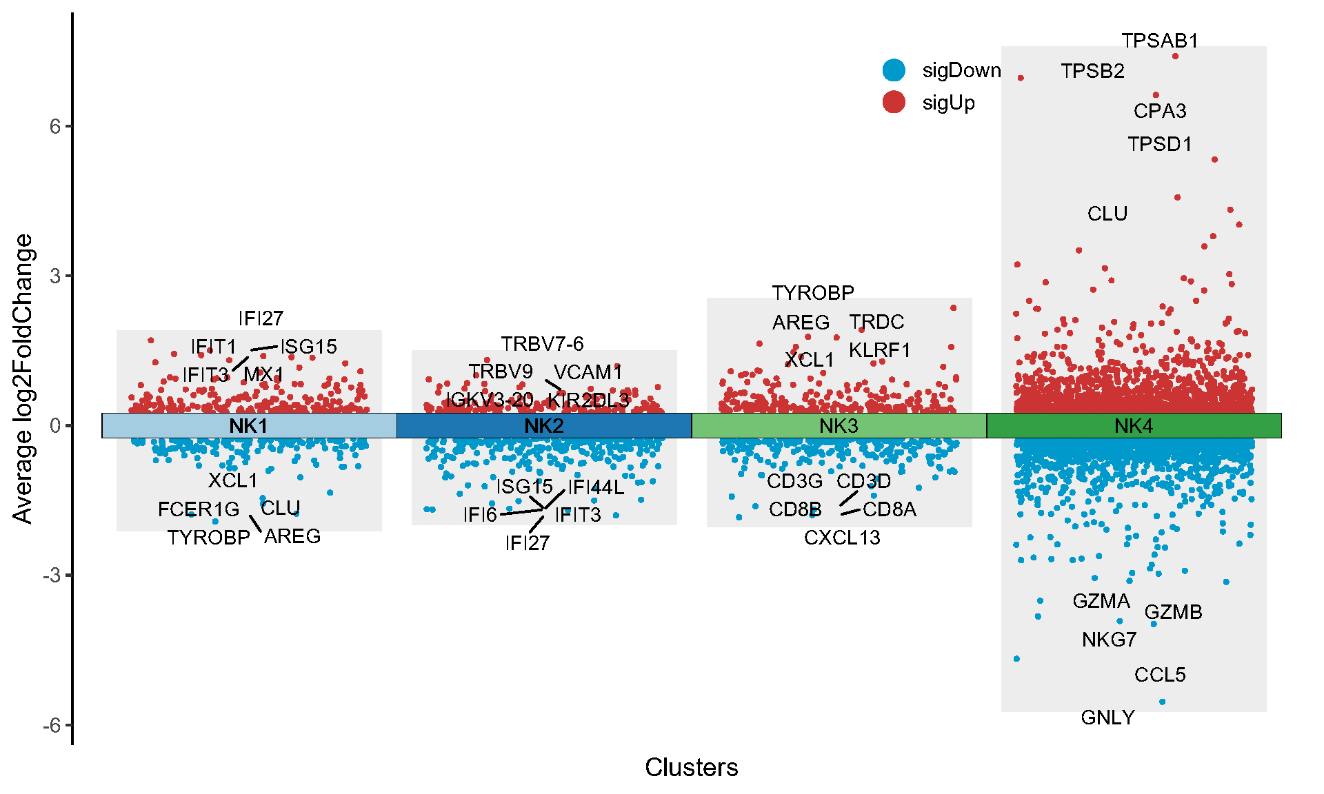
Fig.3.B scRNA volcano

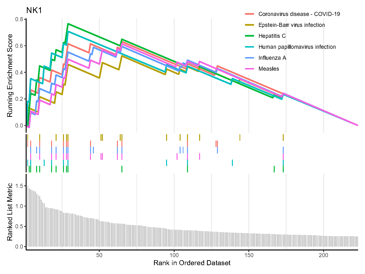
Fig.3.C GSEA结果显示,NK1亚群激活了自然杀伤细胞介导的细胞毒性。NK2,NK3不再重复复现过程。

4.5 NK细胞亚群细胞通讯分析

1
2
3
4
5
6
7
8
9
10
11
12
13
14
15
16
17
18
19
20
21
22
23
24
25
26
27
28
29
30
31
32
33
34
35
36
37
38
39
devtools::install_github('immunogenomics/presto')
rm(list = ls())
NK_subtype <- readRDS('NK_subtype.RDS')
# cellchat
# Step1.创建cellchat对象
data.input <- NK_subtype@assays$RNA@data
meta.data <- NK_subtype@meta.data

cellchat <- createCellChat(object=data.input,
meta = meta.data,
group.by='type')
cellchat <- addMeta(cellchat,meta = meta.data)

# Step2.加载CellChatDB数据库
cellchatDB <- CellChatDB.human
cellchat@DB <- cellchatDB

# Step3.处理表达数据
cellchat <- subsetData(cellchat)
cellchat <- identifyOverExpressedGenes(cellchat,do.fast = FALSE)
cellchat <- identifyOverExpressedInteractions(cellchat)

# Step4.计算通讯概率,推断细胞通讯网络
cellchat <- computeCommunProb(cellchat,population.size = F)
cellchat <- filterCommunication(cellchat,min.cells = 10)

# Step5. 提取预测的细胞通讯网络为data frame
df.net <- subsetCommunication(cellchat)
df.pathway <- subsetCommunication(cellchat,slot.name = 'netP')

# Step6. 在信号通路水平推断细胞通讯
cellchat <- computeCommunProbPathway(cellchat)
# Step7. 计算加和的cell-cell通讯网络
cellchat <- aggregateNet(cellchat)
saveRDS(cellchat,file = 'cellchat.RDS')

levels(cellchat@idents)
netVisual_bubble(cellchat, sources.use = c(1),
targets.use = c(2,3,4,5),remove.isolate = FALSE)

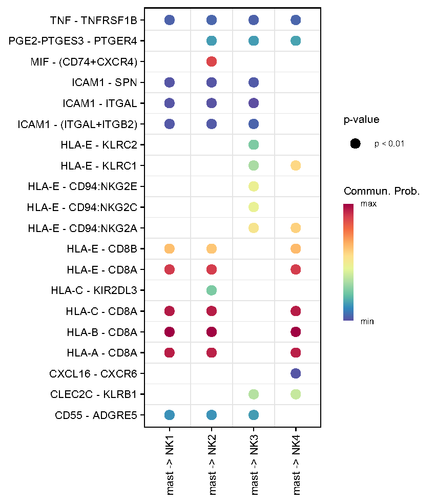
Fig.3.F 肥大细胞和 NK1-3 亚群之间的细胞间相互作用。

4.6 NK细胞耗竭标志物的表达

1
2
3
VlnPlot(NK_subtype,features = c('KLRF1','IL7R','ZNF683','TPSAB1',
'LGALS9','CD44','PTPRC','HAVCR2','NKG7','TIGIT',
'LAG3','CTLA4'),group.by = 'type',pt.size = 0)

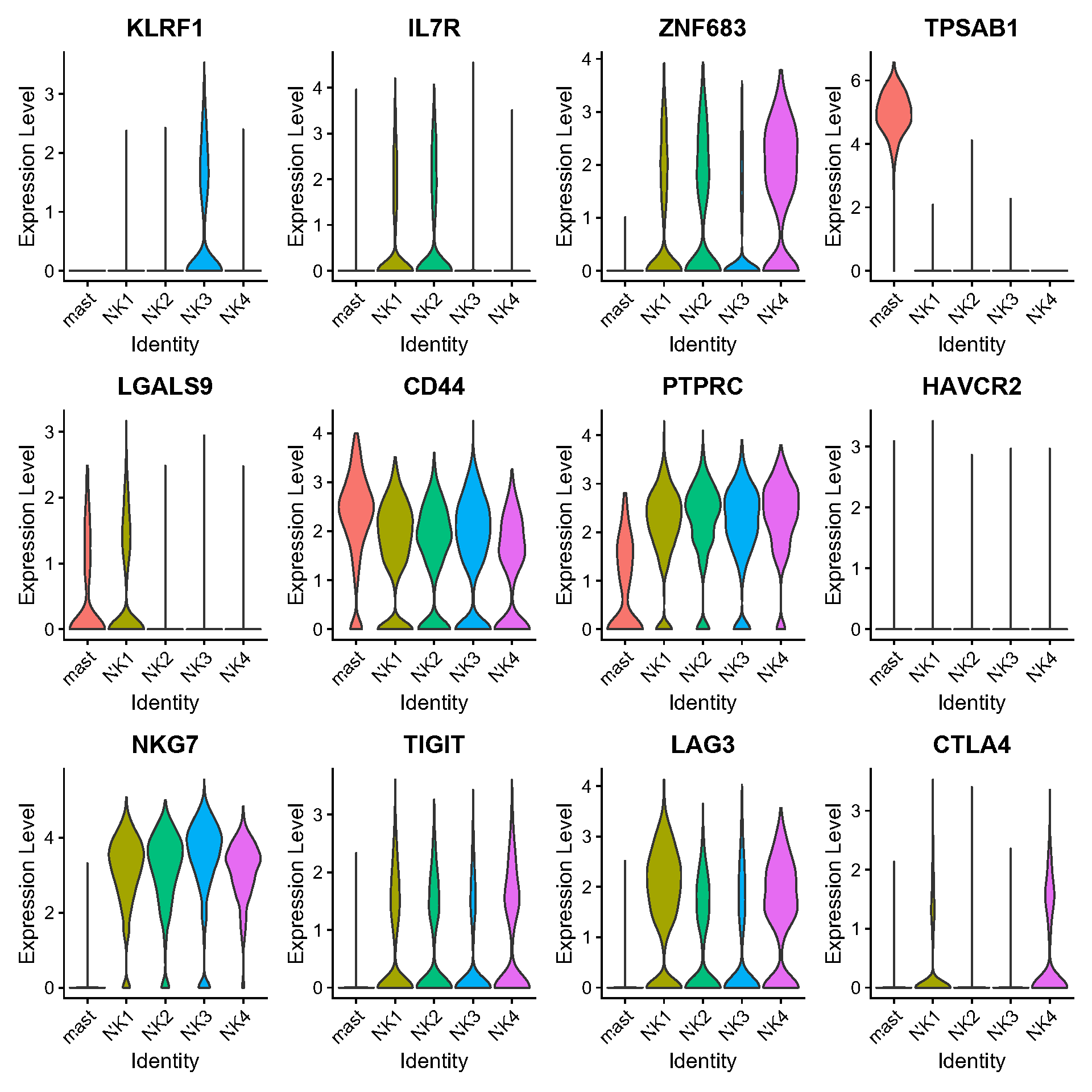
Fig.3.G 细胞耗竭标志物的表达:NK1-3亚群中HAVCR2、TIGIT、LAG3和CTLA4,其中NK3的TIGIT和LAG3表达最高,HAVCR2和CTLA4的部分表达。此外,NK3 的 ZNF683 表达最高。

4.7 GSE150825鼻炎淋巴增生分析

1
2
3
4
5
6
7
8
9
10
11
12
13
14
15
16
17
18
19
20
21
22
23
24
25
26
27
28
29
30
31
32
33
34
35
36
37
38
39
40
41
42
43
44
45
46
47
48
49
50
51
52
rm(list = ls())
gc()
setwd("C:\\Users\\汐\\Desktop\\R语言复现\\NK细胞耗竭和肿瘤细胞进化轨迹")
# 150825,这一步需去前缀GSE150825_
data_150825 <- CreateSeuratObject(counts = Read10X('rawdata/GSE150825_RAW/rawdata/'),
min.cells = 3, min.features = 200)
dim(data_150825)
head(data_150825@meta.data)

# 降维
data_150825 <- NormalizeData(data_150825)
data_150825 <- FindVariableFeatures(data_150825)
data_150825 <- ScaleData(data_150825)
data_150825 <- RunPCA(data_150825)
ElbowPlot(data_150825,ndims = 30)
# 分群
data_150825 <- RunTSNE(data_150825,reduction = 'pca',dims = 1:10)
DimPlot(data_150825,reduction = 'tsne',label = T)
data_150825 <- FindNeighbors(data_150825,dims = 1:10)
data_150825 <- FindClusters(data_150825,resolution = 0.6)
DimPlot(data_150825,reduction = 'tsne',label = T,group.by = 'seurat_clusters')

DotPlot(data_150825,features = c('CD14', 'CD68', 'CD163', 'ITGAX','FCGR3A'))

cell_type <- data.frame(cluster = 0:19,type = 0:19)
cell_type[cell_type$cluster %in% c(1,3,4,5,7,9),'type'] <- 'T cells'
cell_type[cell_type$cluster %in% c(3,5,7,11),'type'] <- 'NK cell'
cell_type[cell_type$cluster %in% c(8,18),'type'] <- 'Myeloid cells'
cell_type[cell_type$cluster %in% c(13,17),'type'] <- 'Epithelial cells'
cell_type[cell_type$cluster %in% c(0,2,6,10,12,16),'type'] <- 'B cells'
cell_type[cell_type$cluster %in% c(6,19),'type'] <- 'plasma cells'
cell_type[cell_type$cluster %in% c(14),'type'] <- 'mast cells'
cell_type[cell_type$cluster %in% c(15),'type'] <- 'fiberblast'

data_150825@meta.data$type <- unlist(lapply(data_150825@meta.data$seurat_clusters,function(x){cell_type[cell_type$cluster==x,'type']}))
DimPlot(data_150825,reduction = 'tsne',group.by = 'type',label = T)

data_150825_nk <- subset(data_150825,subset= type == 'NK cell')

data_150825_nk <- NormalizeData(data_150825_nk)
data_150825_nk <- FindVariableFeatures(data_150825_nk)
data_150825_nk <- ScaleData(data_150825_nk)
data_150825_nk <- RunPCA(data_150825_nk)
ElbowPlot(data_150825_nk,ndims = 30)
data_150825_nk <- RunTSNE(data_150825_nk,reduction = 'pca',dims = 1:20)
DimPlot(data_150825_nk,reduction = 'tsne')
data_150825_nk <- FindNeighbors(data_150825_nk,dims = 1:20)
data_150825_nk <- FindClusters(data_150825_nk,resolution = 0.1)
DimPlot(data_150825_nk,reduction = 'tsne',group.by = 'seurat_clusters',label = T)
data_150825_nk$type <- sapply(data_150825_nk$seurat_clusters, function(x){paste0('NK',as.numeric(x))})
DimPlot(data_150825_nk,reduction = 'tsne',group.by = 'type',label = T)
FeaturePlot(data_150825,features = c('TIGIT','LAG3','NKG7','HAVCR2','ZNF683'))

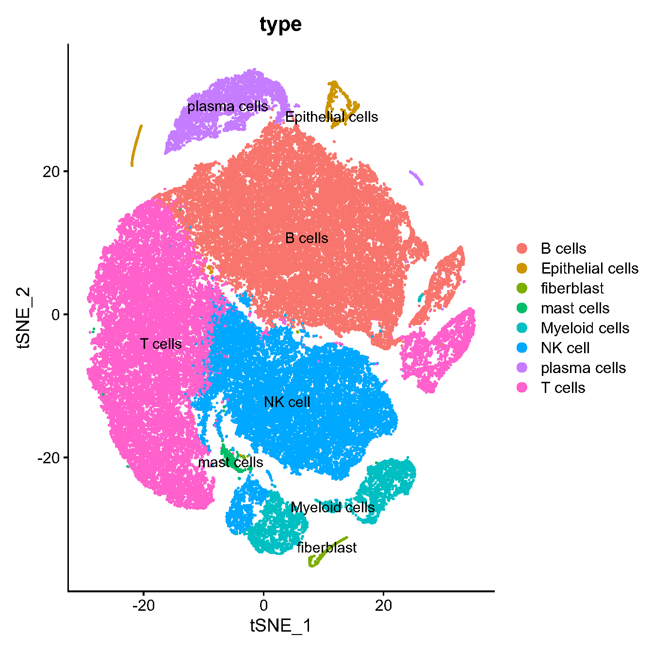
Fig.3.I GSE150825数据集中的NK细胞被缩小并聚类为五个细胞亚群,NK1-5。

Fig3.J

Fig.3.J NKG7、ZNF683、TIGIT、HAVCR2、LAG3和CTLA4在NK1-5亚群中的表达,其中NK-NPC的NK3亚群中ZNF683、TIGIT和LAG3的表达相对较高。

Fig3.K

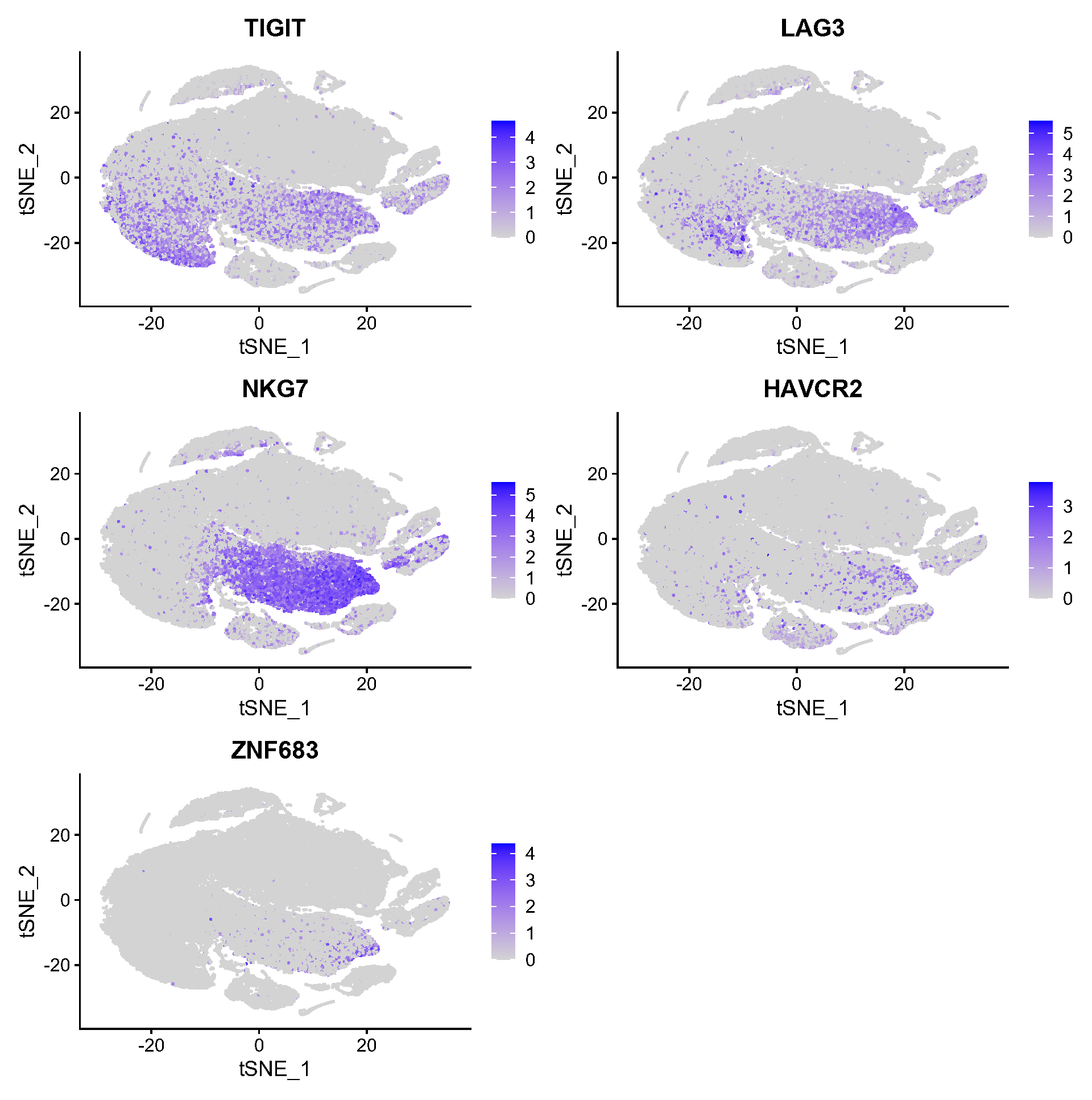
Fig.3.K 数据集没有找到对应的分组信息,找不到NLH组和NPC组。

4.8 对NK-NPC 单细胞谱进行全局细胞间通讯测定

1
2
3
4
5
6
7
8
9
10
11
12
13
14
15
16
17
18
19
20
21
22
23
24
25
26
27
28
29
30
31
32
33
34
35
36
37
38
39
40
41
42
43
44
45
46
47
48
49
50
51
52
53
54
55
56
57
58
59
60
61
62
63
64
65
66
67
68
69
70
71
72
73
74
75
76
77
78
79
80
81
82
83
84
85
86
87
88
89
90
91
92
93
94
95
96
97
98
99
100
101
102
103
104
105
106
107
108
109
110
111
112
113
114
115
116
117
rm(list = ls())
data_162025 <- readRDS("data_162025_type.RDS")
# all cellchat
data.input <- data_162025@assays$RNA@data
meta.data <- data_162025@meta.data
cellchat <- createCellChat(object=data.input,
meta = meta.data,
group.by='type')
cellchat <- addMeta(cellchat,meta = meta.data)
cellchatDB <- CellChatDB.human
cellchat@DB <- cellchatDB
cellchat <- subsetData(cellchat)
cellchat <- identifyOverExpressedGenes(cellchat,do.fast = FALSE)
cellchat <- identifyOverExpressedInteractions(cellchat)
cellchat <- computeCommunProb(cellchat,population.size = F)
cellchat <- filterCommunication(cellchat,min.cells = 10)
df.net <- subsetCommunication(cellchat)
df.pathway <- subsetCommunication(cellchat,slot.name = 'netP')
cellchat <- computeCommunProbPathway(cellchat)
cellchat <- aggregateNet(cellchat)
netVisual_bubble(cellchat, sources.use = c(1,2,4,6),
targets.use = c(4,5,6),signaling = 'GALECTIN',remove.isolate = FALSE)

# Epithelial subtype
Epi_sub <- subset(data_162025,subset=type=='Epithelial cells')
Epi_sub <- NormalizeData(Epi_sub)
Epi_sub <- FindVariableFeatures(Epi_sub)
Epi_sub <- ScaleData(Epi_sub)
Epi_sub <- RunPCA(Epi_sub)
ElbowPlot(Epi_sub,ndims = 30)
Epi_sub <- RunTSNE(Epi_sub,reduction = 'pca',dims = 1:20)
DimPlot(Epi_sub,reduction = 'tsne')
Epi_sub <- FindNeighbors(Epi_sub,dims = 1:20)
Epi_sub <- FindClusters(Epi_sub,resolution = 0.3)
DimPlot(Epi_sub,reduction = 'tsne',group.by = 'seurat_clusters',label = T)
Epi_sub$type <- sapply(Epi_sub$seurat_clusters, function(x){paste0('Epi',as.numeric(x))})

DimPlot(Epi_sub,reduction = 'tsne',group.by = 'type',label = T,label.box = T)
dim(Epi_sub)

# copycat
# 鉴定正常细胞和肿瘤细胞
Epi_cnv <- copykat(rawmat=Epi_sub@assays$RNA@counts, id.type="S", ngene.chr=5, win.size=25,
KS.cut=0.1, sam.name="Epi_sub", distance="euclidean", norm.cell.names="",
output.seg="FLASE", plot.genes="TRUE", genome="hg20",n.cores=1)

saveRDS(Epi_cnv,file = 'Epi_cnv.RDS')
Epi_cnv <- readRDS('Epi_cnv.RDS')

pred.test <- data.frame(Epi_cnv$prediction)
pred.test <- pred.test[-which(pred.test$copykat.pred=="not.defined"),] ##remove undefined cells
CNA.test <- data.frame(Epi_cnv$CNAmat)
head(pred.test)
head(CNA.test[ , 1:5])
Epi_sub@meta.data$copykat.pred <- ifelse(rownames(Epi_sub@meta.data) %in% rownames(pred.test[pred.test$copykat.pred=='aneuploid',]),'aneuploid',
ifelse(rownames(Epi_sub@meta.data) %in% rownames(pred.test[pred.test$copykat.pred=='diploid',]),'diploid',NA)
)

my_palette <- colorRampPalette(rev(RColorBrewer::brewer.pal(n = 3, name = "RdBu")))(n = 999)

chr <- as.numeric(CNA.test$chrom) %% 2+1
rbPal1 <- colorRampPalette(c('black','grey'))
CHR <- rbPal1(2)[as.numeric(chr)]
chr1 <- cbind(CHR,CHR)

rbPal5 <- colorRampPalette(RColorBrewer::brewer.pal(n = 8, name = "Dark2")[2:1])
com.preN <- pred.test$copykat.pred
pred <- rbPal5(2)[as.numeric(factor(com.preN))]

cells <- rbind(pred,pred)
col_breaks = c(seq(-1,-0.4,length=50),seq(-0.4,-0.2,length=150),
seq(-0.2,0.2,length=600),seq(0.2,0.4,length=150),seq(0.4, 1,length=50))
pdf("Fig4_C.pdf",width=15,height=10)
heatmap.3(t(CNA.test[,4:ncol(CNA.test)]),dendrogram="r",
distfun = function(x) parallelDist::parDist(x,threads =4, method = "euclidean"),
hclustfun = function(x) hclust(x, method="ward.D2"),
ColSideColors=chr1,RowSideColors=cells,Colv=NA, Rowv=TRUE,
notecol="black",col=my_palette,breaks=col_breaks, key=TRUE,
keysize=1, density.info="none", trace="none",
cexRow=0.1,cexCol=0.1,cex.main=1,cex.lab=0.1,
symm=F,symkey=F,symbreaks=T,cex=1, cex.main=4, margins=c(10,10))
legend("topright", paste("pred.",names(table(com.preN)),sep=""), pch=15,col=RColorBrewer::brewer.pal(n = 8, name = "Dark2")[2:1], cex=0.6, bty="n")
dev.off()
# 鉴定肿瘤细胞亚型
tumor.cells <- pred.test$cell.names[which(pred.test$copykat.pred=="aneuploid")]
tumor.mat <- CNA.test[, which(colnames(CNA.test) %in% tumor.cells)]
hcc <- hclust(parallelDist::parDist(t(tumor.mat),threads =4, method = "euclidean"), method = "ward.D2")
hc.umap <- cutree(hcc,2)

rbPal6 <- colorRampPalette(RColorBrewer::brewer.pal(n = 8, name = "Dark2")[3:4])
subpop <- rbPal6(2)[as.numeric(factor(hc.umap))]
cells <- rbind(subpop,subpop)
pdf("Fig4_D.pdf",width=15,height=10)
heatmap.3(t(tumor.mat),dendrogram="r", distfun = function(x) parallelDist::parDist(x,threads =4, method = "euclidean"), hclustfun = function(x) hclust(x, method="ward.D2"),
ColSideColors=chr1,RowSideColors=cells,Colv=NA, Rowv=TRUE,
notecol="black",col=my_palette,breaks=col_breaks, key=TRUE,
keysize=1, density.info="none", trace="none",
cexRow=0.1,cexCol=0.1,cex.main=1,cex.lab=0.1,
symm=F,symkey=F,symbreaks=T,cex=1, cex.main=4, margins=c(10,10))
legend("topright", c("c1","c2"), pch=15,col=RColorBrewer::brewer.pal(n = 8, name = "Dark2")[3:4], cex=0.9, bty='n')
dev.off()

Epi_sub@meta.data$copykat.Tumor_pred <- ifelse(colnames(Epi_sub) %in% names(hc.umap[hc.umap==1]),'tumor cluster1',
ifelse(colnames(Epi_sub) %in% names(hc.umap[hc.umap==2]),'tumor cluster2','normal'))
p1 <- DimPlot(Epi_sub,group.by = 'type',label = T)
p2 <- DimPlot(Epi_sub,group.by = 'copykat.pred',label = T)
p3 <- DimPlot(Epi_sub,group.by = 'copykat.Tumor_pred',label=T)
pdf("Fig4_E.pdf",width=21,height=7)
p1+p2+p3
dev.off()
pdf("Fig4_F.pdf",width=9,height=6)
DotPlot(Epi_sub,features = c('LGALS9','HLA-A','HLA-B','HLA-C','HLA-E','HLA-F','HLA-G','B2M'),group.by = 'copykat.Tumor_pred')
dev.off()
pdf("Fig4_G.pdf",width=10,height=10)
# EBV感染相关蛋白在两类细胞中的表达
FeaturePlot(Epi_sub,features = c('KRT5','SSTR2','LMP-1/BNLF2a/b','RPMS1/A73'))
dev.off()

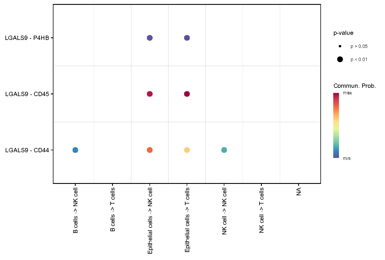
Fig.4.A 所有细胞类型之间关于半乳糖凝集素信号传导的细胞间相互作用。

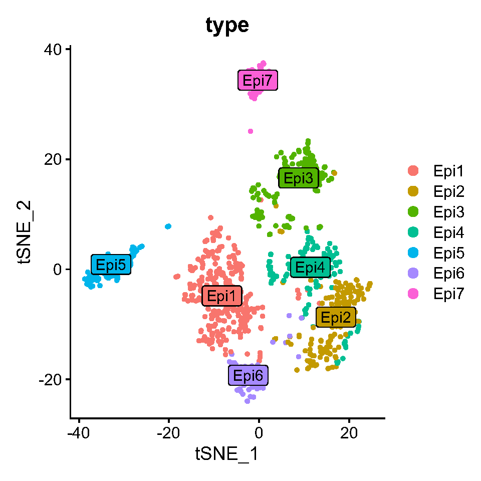
Fig.4.B Epi1-7 细胞亚群是通过上皮细胞的降维和聚类获得的。

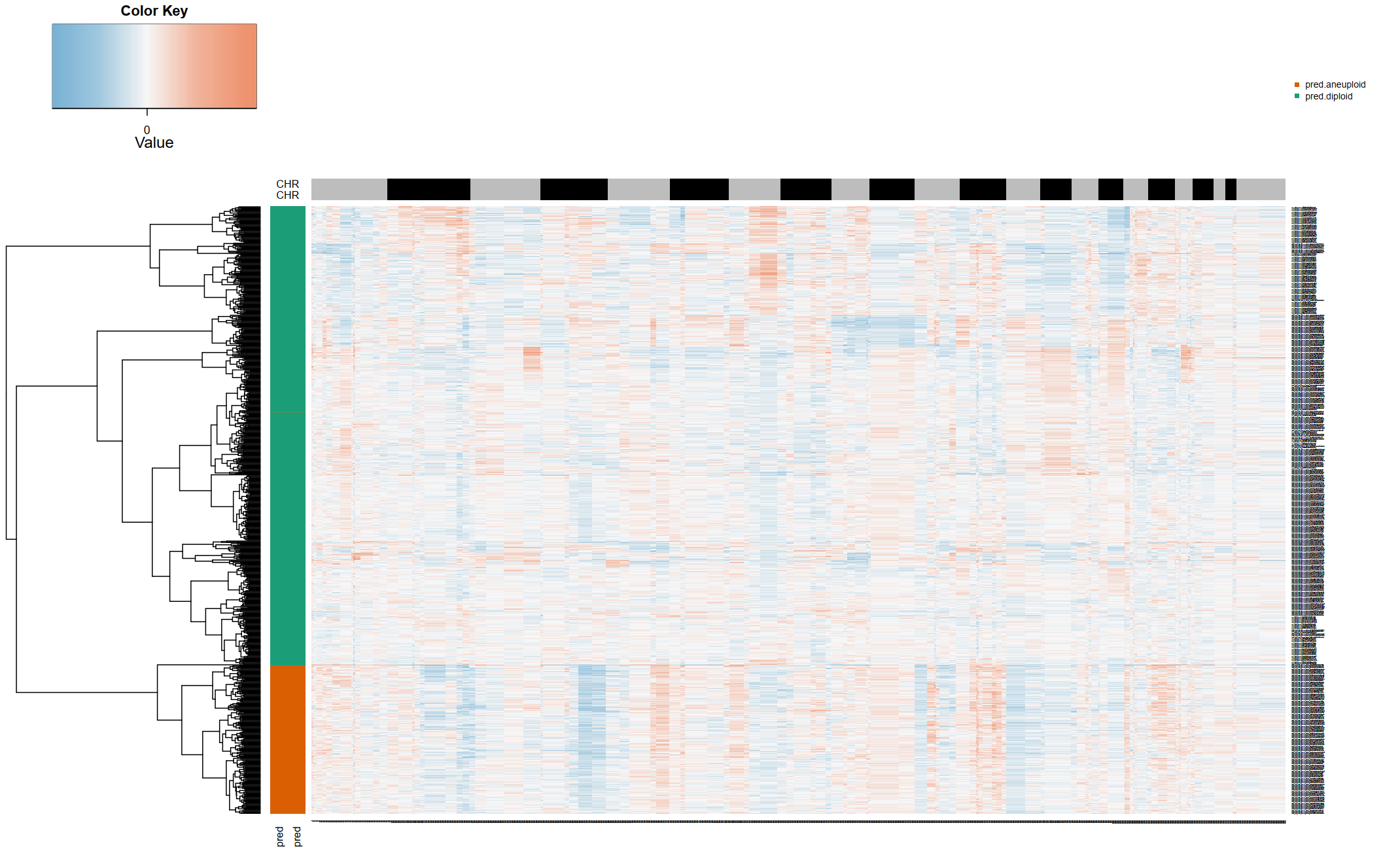
Fig.4.C copykat软件识别良恶性上皮细胞,橙色代表拷贝数增加,蓝色代表拷贝数缺失,上面穿插的灰色和黑色代表不同的染色体;Pred.Aneuploid:恶性;pred.diploid:良性。

Fig4_D

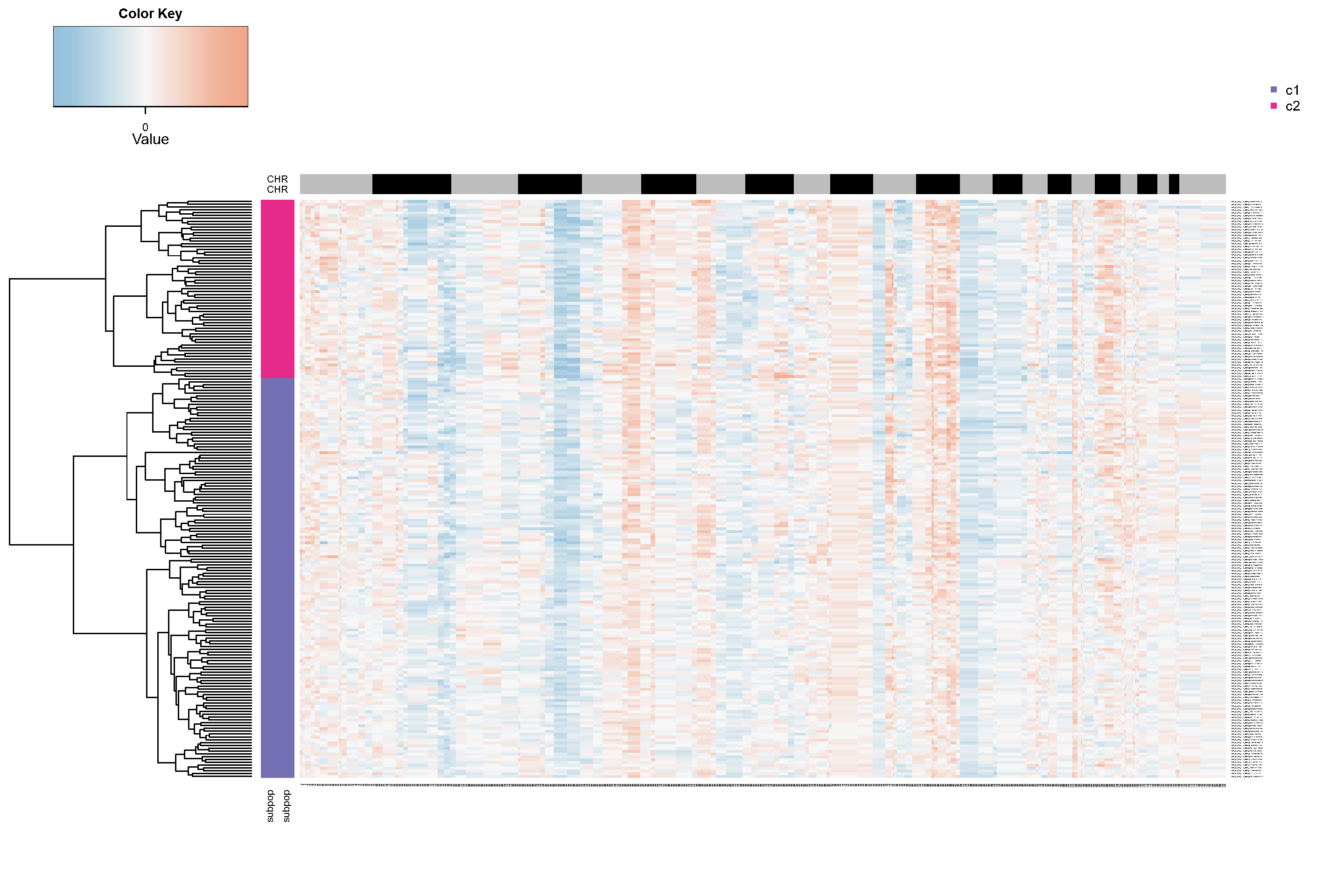
Fig.4.D copykat 软件进一步将恶性肿瘤细胞识别为两种亚型,即肿瘤亚型 1 和肿瘤亚型 2。

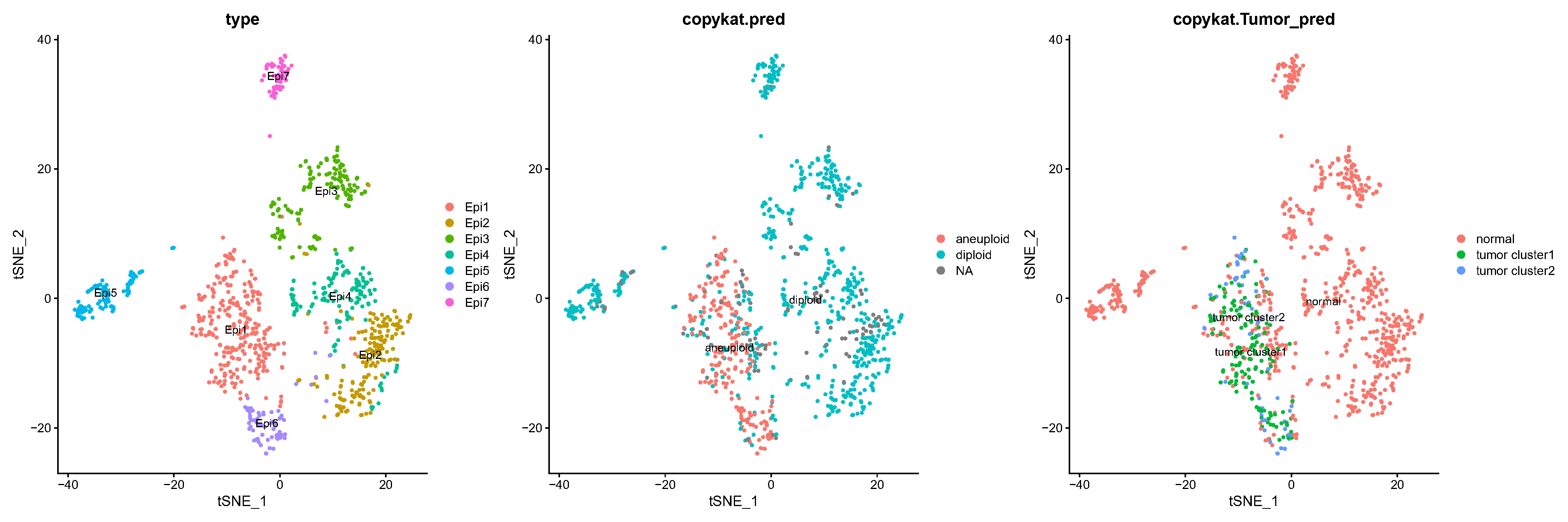
Fig.4.E 肿瘤亚型 1 和肿瘤亚型 2 两种亚型在 TNSE 图中绘制。

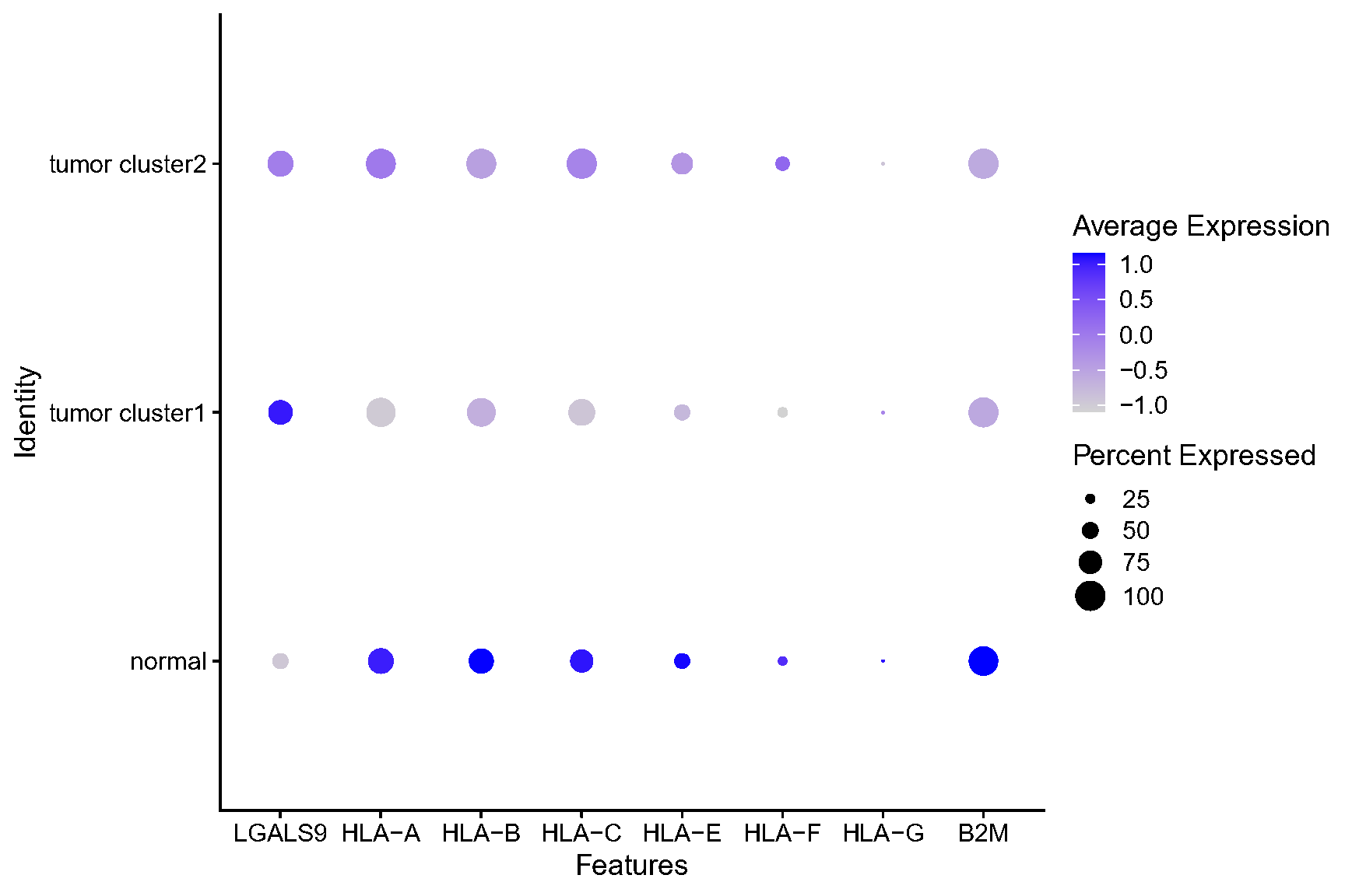
Fig.4.F LGALS9 和 MHC I 类分子在肿瘤亚型 1 和肿瘤亚型 2 中的表达。

Fig4_G

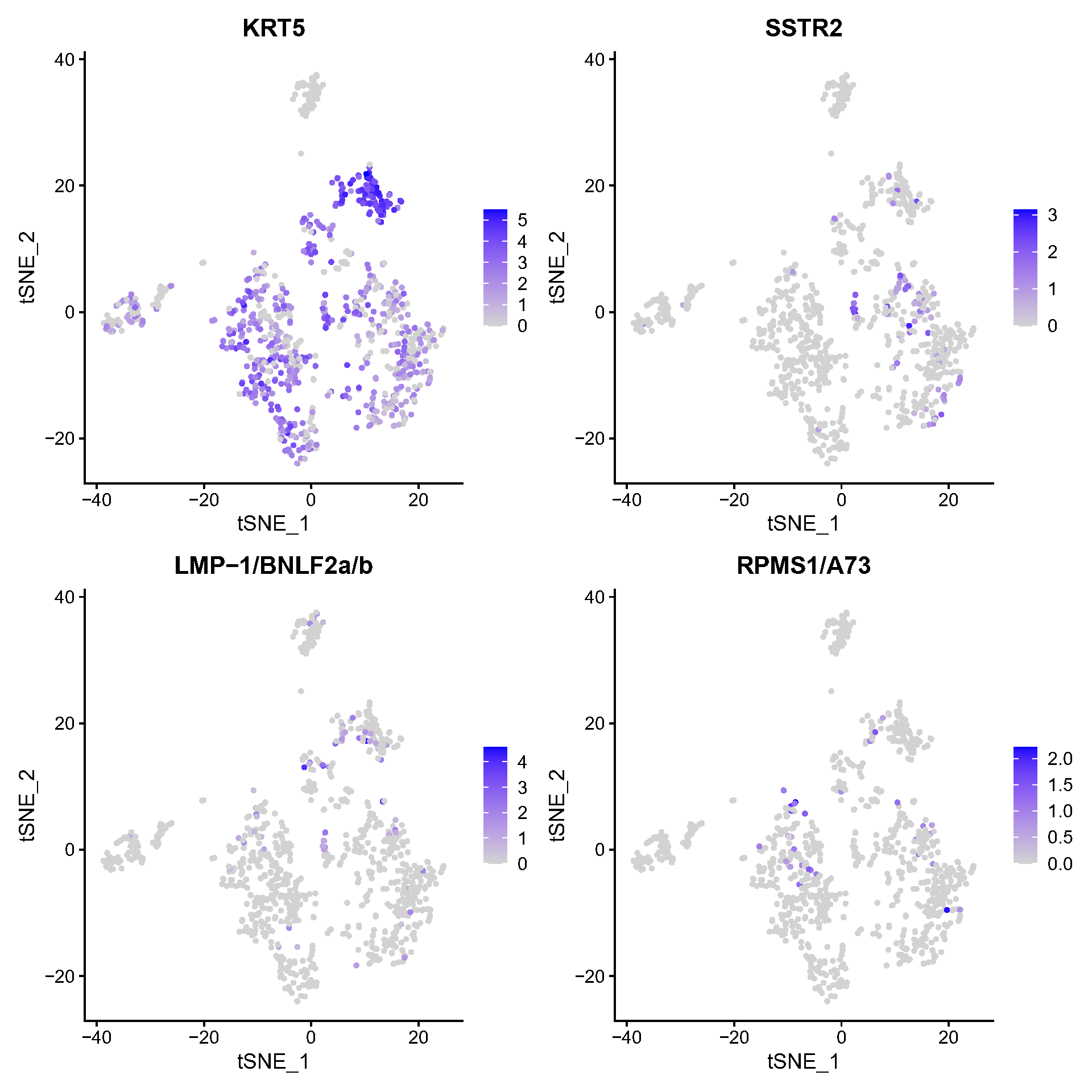
Fig.4.G KRT5、SSTR2、LMP-1/BNLF2a/b和RPMS1/A73在肿瘤亚型1和肿瘤亚型2中的表达和分布。

4.9 NK-NPCtumor1 亚群细胞进化轨迹和功能富集分析

1
2
3
4
5
6
7
8
9
10
11
12
13
14
15
16
17
18
19
20
21
22
23
24
25
26
27
28
29
30
31
32
33
34
35
36
37
38
39
40
41
42
43
44
45
46
47
48
49
50
51
52
53
# tumor1 亚群
tumor1_sub <- Epi_sub[, Epi_sub@meta.data$copykat.Tumor_pred == 'tumor cluster1', ]

tumor1_sub <- NormalizeData(tumor1_sub)
tumor1_sub <- FindVariableFeatures(tumor1_sub)
tumor1_sub <- ScaleData(tumor1_sub)
tumor1_sub <- RunPCA(tumor1_sub)
ElbowPlot(tumor1_sub,ndims = 30)
tumor1_sub <- RunTSNE(tumor1_sub,reduction = 'pca',dims = 1:20)
DimPlot(tumor1_sub,reduction = 'tsne')
tumor1_sub <- FindNeighbors(tumor1_sub,dims = 1:20)
tumor1_sub <- FindClusters(tumor1_sub,resolution = 0.8)
DimPlot(tumor1_sub,reduction = 'tsne',group.by = 'seurat_clusters',label = T)
tumor1_sub$type <- sapply(tumor1_sub$seurat_clusters, function(x){paste0('Epi',as.numeric(x))})

# SCORPIUS 拟时序
group_name <- as.numeric(as.factor(tumor1_sub@meta.data$type))
names(group_name) <- tumor1_sub@meta.data$type
group_name <- as.factor(group_name)

space <- reduce_dimensionality(t(tumor1_sub@assays$RNA@data), "spearman")
draw_trajectory_plot(space,group_name, contour = TRUE)

traj <- infer_trajectory(space)
draw_trajectory_plot(space, group_name, traj$path, contour = TRUE)

gimp <- gene_importances(
t(tumor1_sub@assays$RNA@scale.data),
traj$time,
num_permutations = 10,
num_threads = 8,
ntree = 10000,
ntree_perm = 1000
)
gimp$qvalue <- p.adjust(gimp$pvalue, "BH", length(gimp$pvalue))
gene_sel <- gimp$gene[gimp$qvalue < .05]
expr_sel <- scale_quantile(t(tumor1_sub@assays$RNA@scale.data)[,gene_sel])
time <- traj$time
draw_trajectory_heatmap(expr_sel, time,progression_group=group_name)

# tumor1 差异
tumor1_sub_markers <- FindAllMarkers(tumor1_sub)
tumor1_sub_markers$cluster <- sapply(tumor1_sub_markers$cluster, function(x){paste0('Epi',as.numeric(x))})
jjVolcano(tumor1_sub_markers)
VlnPlot(tumor1_sub,features = c('KRT5','VIM','SSTR2','LMP-1/BNLF2a/b','RPS18','RPS23'))

tumor1_sub_deg <- tumor1_sub_markers[tumor1_sub_markers$cluster=='Epi1',]
tumor1_sub_marker <- tumor1_sub_deg$avg_log2FC
names(tumor1_sub_marker) <- bitr(tumor1_sub_deg$gene,fromType = 'SYMBOL',toType = 'ENTREZID',OrgDb = org.Hs.eg.db)[,'ENTREZID']
tumor1_sub_marker <- sort(tumor1_sub_marker,decreasing = T)

tumor1 <- gseKEGG(tumor1_sub_marker)
gseaplot2(tumor1,geneSetID = 2)

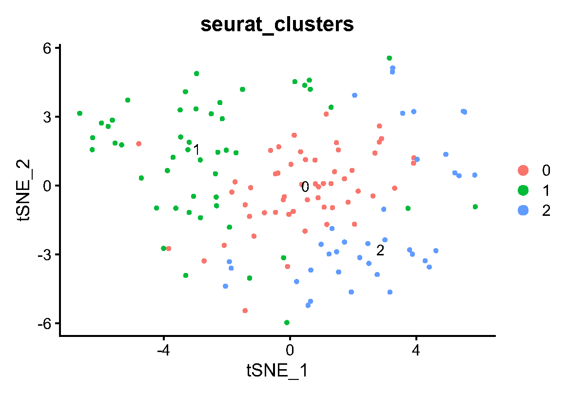
Fig.5.A Epi T1-4 细胞亚群是通过肿瘤亚型 1 亚群的降维和聚类获得的。

Fig5.B3

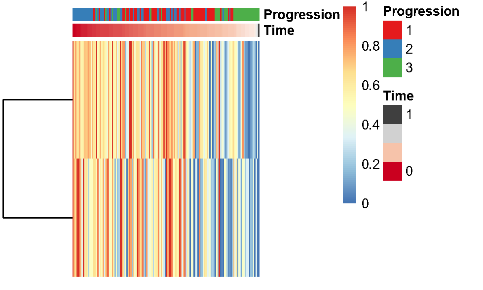
Fig.5.B 考虑到EBV活性状态对tumor1可能有影响,于是把tumor1单拎出来进行拟时序分析,这里就随便选一个亚群了。

Fig5.B Fig5.B2

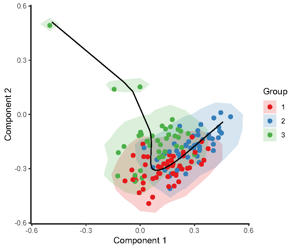
Fig.5.B 拟时序分析,肿瘤亚型1的细胞进化轨迹:从0到1的时间,上皮细胞进化轨迹方向从Epi T1-Epi T4,对应全局基因表达变化。红色表示高表达,蓝色表示低表达。

Fig5.C

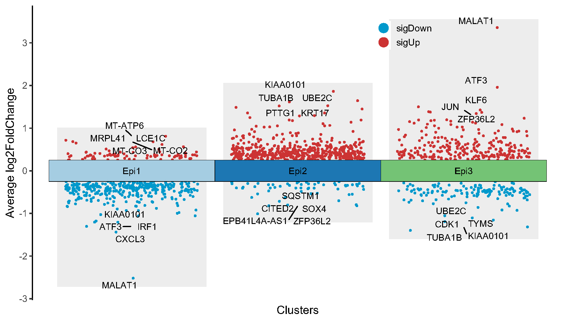
Fig.5.C Epi T1-4 亚群的标记基因

Fig5.D

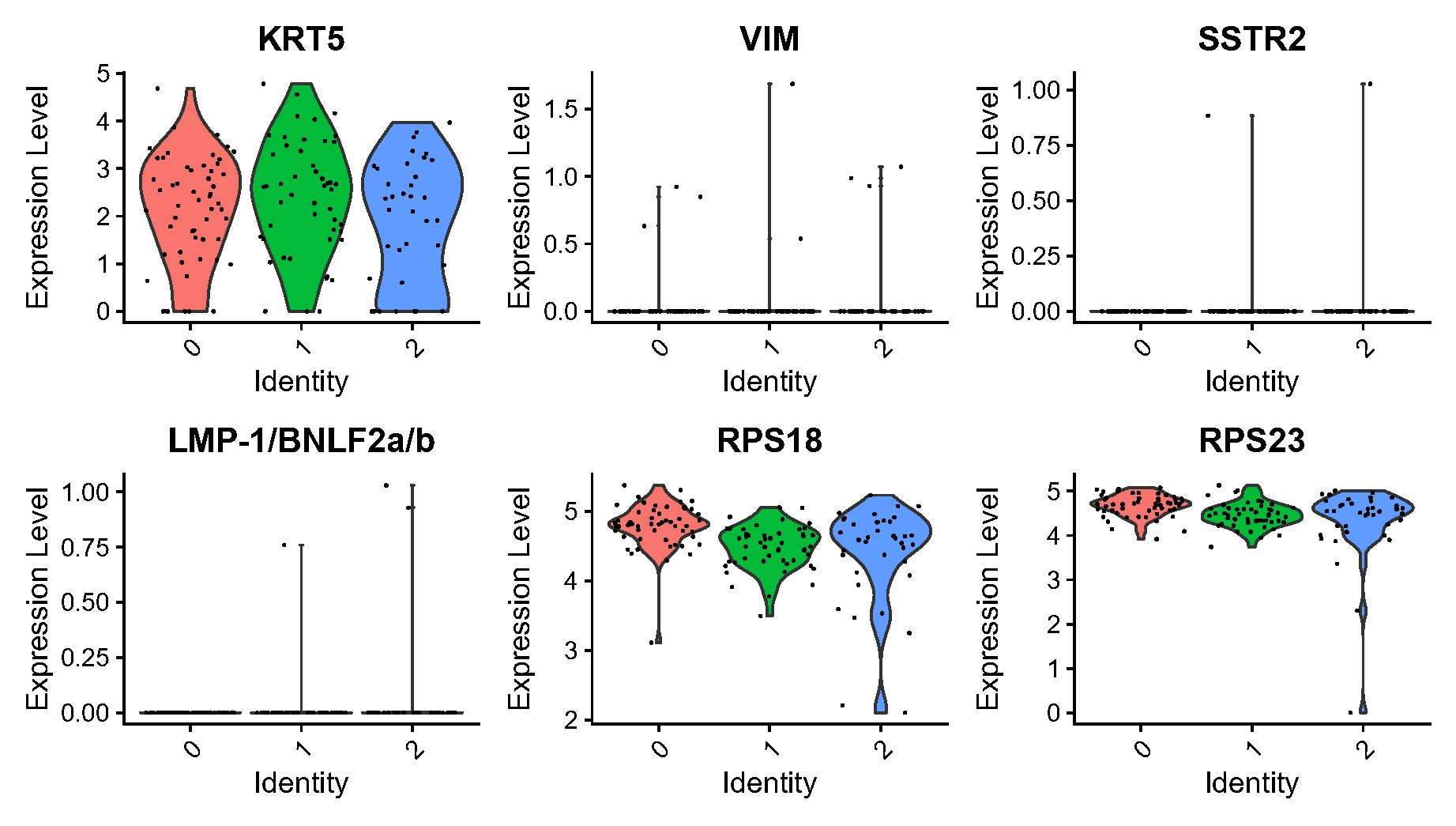
Fig.5.D Violin 图显示了 Epi T1-T4 亚群中 KRT5、VIM、SSTR2、LMP-1/BNLF2a/b、RPS18 和 RPS23 基因的表达及其变异变化。

Fig5.E

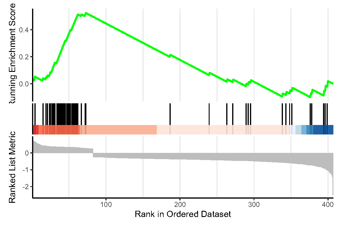
Fig.5.E 亚群各标记基因的 GSEA 富集分析。

5 结论

综上所述,本研究揭示了NK-NPC的NK细胞耗竭情况。肿瘤细胞可能通过产生与NK细胞表面的抑制性受体结合的负配体来诱导NK细胞的功能抑制和耗竭。此外,肿瘤细胞可能通过NK-NPC中LGALS9的表达来抑制NK细胞的功能。本研究首次进一步确定了NK-NPC中EBV活性状态下肿瘤细胞的独特进化轨迹。我们的研究结果为不同阶段的肿瘤监测提供了潜在的治疗靶点和可能的生物标志物,从而提高了NK-NPC患者的生存率。然而,还需要进一步的功能实验来研究潜在的机制。

6 复现心得

  1. RDS vs. RData vs. RDA:

    格式 用途 优点 缺点
    RData 保存整个 R 环境 快速加载和保存整个 R 环境 文件大小大
    RDA 保存单个 R 对象 储存大型对象有效 只保存单个对象
    RDS 保存二进制序列化的 R 对象 文件大小小,加载速度快,跨平台兼容 只适用于 R 对象
  2. 当某一流程为限速步骤时,最好能将结果对象保存为文件,以便需要时可再次读入。

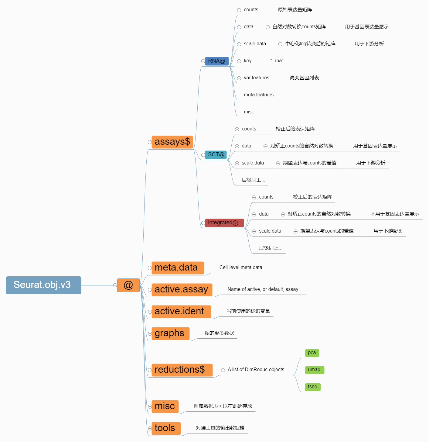
  3. Seurat对象中储存了关于这个单细胞项目的几乎所有信息,包括每个细胞的barcodes,原始表达矩阵以及运行过哪些分析等,后续对单细胞的分群注释等信息都是保存在Seurat对象中的。在R中可以使用str()函数查看数据结构。


一篇基于R语言的scRNA-seq文章复现
http://horizongazer.github.io/2024/05/20/一篇基于R语言的scRNA-seq文章复现/
作者
HorizonGazer
发布于
2024年5月20日
许可协议